Image Classifier with Streaming Augmented Images from Local Storage

Gargeya Sharma 15 Jun, 2021 • 5 min read

This article was published as a part of the Data Science Blogathon

Introduction

Storing a huge amount of image data on the memory before training is tedious. When we are working with a lot of data, oftentimes these problems occur, when either the machine gets slow, how buffer memory gets overloaded and training gets crashed, etc.

The point is that usually, with a small amount of data that available with `tf.data` or other open resources we don’t feel the need to stream data directly from the local storage rather than first loading all the images in form of tensors and then using those for the computer vision model training.

With this technique of creating an ImageDataGenerator (similar to a python generator, which doesn’t load the data beforehand in the memory and iterates only when required or asked), Tensorflow has is an amazing method, where you can do the same with images and that’s not even the best part, on top of loading images, you can apply different augmentations post-loading those images so that you can train your model with more diverse training examples.

Objective

Today, we will look at a simple code that does exactly that on the “Horses and Human dataset”. In case you wonder about doing Image classification on the same dataset using Tensorflow Data Pipelines( I highly recommend checking it out), check out this blog by me written earlier for the same: Image Classification with TensorFlow Data Pipelines.

You can get the Training_data and Validation_data from their respective links as a zip file. Although with colab notebooks, we are directly downloading the data through these links in the first code cell itself.

Dataset is created by Laurence Cemorony, for more details on the dataset check out this link. In brief, The dataset contains 500 computerized rendered pictures of different types of horses in numerous postures in various areas. It additionally contains 527 computerized rendered pictures of Humans for various postures and backgrounds.

Implementation

Let’s look at the preparation code first before creating an ImageDataGenerator

Step 1

Retrieve the Data (Humans and Horse) OR you already have your data with you

!wget --no-check-certificate 
    https://storage.googleapis.com/laurencemoroney-blog.appspot.com/horse-or-human.zip 
    -O /tmp/horse-or-human.zip

## Validation Dataset
!wget --no-check-certificate 
    https://storage.googleapis.com/laurencemoroney-blog.appspot.com/validation-horse-or-human.zip 
    -O /tmp/validation-horse-or-human.zip

Step 2

The next code will set up the downloaded data from a zip file into directories. Remember, each class has its own directory/folder with its folder name as the label for that class, and all its respective images into it.

import os
import zipfile
local_zip = '/tmp/horse-or-human.zip'
zip_ref = zipfile.ZipFile(local_zip, 'r')
zip_ref.extractall('/tmp/horse-or-human')
local_zip = '/tmp/validation-horse-or-human.zip'
zip_ref = zipfile.ZipFile(local_zip, 'r')
zip_ref.extractall('/tmp/validation-horse-or-human')
zip_ref.close()

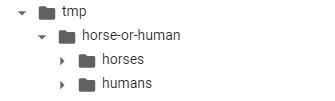
Here is how the File hierarchy would look like:

Step 3

To avoid writing the file path, again and again, we can simply assign them to our current working directory through the following code.

# Directory with our training horse pictures
train_horse_dir = os.path.join('/tmp/horse-or-human/horses')
# Directory with our training human pictures
train_human_dir = os.path.join('/tmp/horse-or-human/humans')
# Directory with our training horse pictures
validation_horse_dir = os.path.join('/tmp/validation-horse-or-human/horses')
# Directory with our training human pictures
validation_human_dir = os.path.join('/tmp/validation-horse-or-human/humans')

Let’s also capture all the file names into these leaf directories (the last level for the folders which contains the images). `os.listdir()` function does exactly that, it gives you a list of items in the folder mentioned as the parameter.

train_horse_names = os.listdir(train_horse_dir)
train_human_names = os.listdir(train_human_dir)
validation_horse_hames = os.listdir(validation_horse_dir)
validation_human_names = os.listdir(validation_human_dir)

Step 4

Setup is completed, now comes the existing part of making the model and letting it train on those images from the local storage using ImageDataGenerator.

Making these data generators is a data preprocessing phase, because every importing, changing shape, size, augmenting, and all is done before feeding it to the neural network.
Here are the light augmentations that we are applying to the raw dataset. We will create 2 generators, one for the training images and the other for validation images. Our actual image size is 300×300, but just to show you guys that it doesn’t matter while we stream these images from local, I am choosing half the original size (150×150).
One more thing that I am changing with the images is that usually, the pixel values in any images are between 0-255, but I am rescaling the images to get all the pixel values between 0-1.

NOTE: ImageDataGenerators can be used in various ways, for today’s topic the function having the spotlight will be .flow_from_directory(directory_name)

import tensorflow as tf
from tensorflow.keras.preprocessing.image import ImageDataGenerator
# All images will be rescaled by 1./255
train_datagen = ImageDataGenerator(rescale=1/255)
validation_datagen = ImageDataGenerator(rescale=1/255)
# Flow training images in batches of 128 using train_datagen generator
train_generator = train_datagen.flow_from_directory(
        '/tmp/horse-or-human/',  # This is the source directory for training images
        target_size=(150, 150),  # All images will be resized to 150x150
        batch_size=128,
        # Since we use binary_crossentropy loss, we need binary labels
        class_mode='binary')
# Flow training images in batches of 128 using train_datagen generator
validation_generator = validation_datagen.flow_from_directory(
        '/tmp/validation-horse-or-human/',  # This is the source directory for training images
        target_size=(150, 150),  # All images will be resized to 150x150
        batch_size=32,
        # Since we use binary_crossentropy loss, we need binary labels
        class_mode='binary')

Step 5

Finally, it’s our model creation time and then training the model using this train_generator and validation_generator. Reminder: Don’t forget to notice the input shape mentioned in the first layer of my model and target shape in the above train_generator part.

model = tf.keras.models.Sequential([
    # Note the input shape is the desired size of the image 150x150 with 3 bytes color
    # This is the first convolution
    tf.keras.layers.Conv2D(16, (3,3), activation='relu', input_shape=(150, 150, 3)),
    tf.keras.layers.MaxPooling2D(2, 2),
    # The second convolution
    tf.keras.layers.Conv2D(32, (3,3), activation='relu'),
    tf.keras.layers.MaxPooling2D(2,2),
    # The third convolution
    tf.keras.layers.Conv2D(64, (3,3), activation='relu'),
    tf.keras.layers.MaxPooling2D(2,2),
    # The fourth convolution
    tf.keras.layers.Conv2D(64, (3,3), activation='relu'),
    tf.keras.layers.MaxPooling2D(2,2),
    # Flatten the results to feed into a DNN
    tf.keras.layers.Flatten(),
    # 512 neuron hidden layer
    tf.keras.layers.Dense(512, activation='relu'),
    # Only 1 output neuron. It will contain a value from 0-1 where 0 for 1 class ('horses') and 1 for the other ('humans')
    tf.keras.layers.Dense(1, activation='sigmoid')
])

Now, as it is binary image classification, we need to use binary_crossentropy as the loss for the best results. For optimizer, I am simply going for RMSprop with a learning rate == 0.001.

from tensorflow.keras.optimizers import RMSprop
model.compile(loss='binary_crossentropy',
              optimizer=RMSprop(learning_rate=0.001),
              metrics=['accuracy'])

Here is how we are gonna make a symphony of all the above steps into a single computer vision model in training. Let’s train for only 15 epochs and observe the metrics.

history = model.fit(
      train_generator,
      steps_per_epoch=8,  
      epochs=15,
      verbose=1,
      validation_data = validation_generator,
      validation_steps=8)

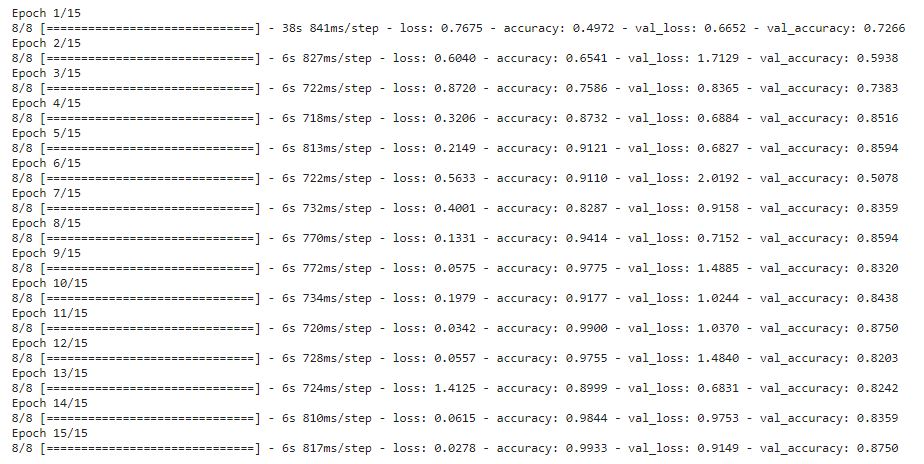
As you can clearly, see the model did great with only 15 epochs, although, with few more training epochs and some additional heavy data augmentation, you can further improve the accuracy. That’s upon you to experiment and enjoy.

Conclusion

This is the end of this article and I hope you got excited the same as I did when I discovered this feature and thought that such things are also available and so easy to implement.

Gargeya Sharma

B.Tech 4th Year Student
Specialized in Deep Learning and Data Science
For getting more info check out my Github Homepage

LinkedIn GitHub

Photo by Solen Feyissa on Unsplash

The media shown in this article are not owned by Analytics Vidhya and are used at the Author’s discretion.

Gargeya Sharma 15 Jun 2021

Deep Learning Image Intermediate Python Unstructured Data