Predictive Modelling – Rain Prediction in Australia With Python

Introduction:

In this article, I will be implementing a predictive model on Rain Dataset to predict whether or not it will rain tomorrow in Australia. The Dataset contains about 10 years of daily weather observations of different locations in Australia. By the end of this article, you will be able to build a predictive model.

So, without further ado, let’s get started.

“Possessed is probably the right word. I often tell people, ‘I don’t want to necessarily be a data scientist. You just kind of are a data scientist. You just can’t help but look at that data set and go, ‘I feel like I need to look deeper. I feel like that’s not the right fit.”

―  Jennifer Shin, Senior Principal Data Scientist at Nielsen; Lecturer at UC Berkeley

Image by Author(Made with Canva)

Table of contents:

1. Problem Statement
2. Data Source
3. Importing Necessary Libraries
4. Data Preprocessing
5. Finding categorical and Numerical features in Dataset
6. Cardinality check for categorical features
7. Handling Missing values
8. Outlier detection and treatment
9. Exploratory Data Analysis
10. Encoding categorical features
11. Correlation
12. Feature Importance
13. Splitting Data into Training and Testing sets
14. Feature Scaling
15. Model Building and Evaluation
16. Results and Conclusion
17. Save Model and Scaling object with Pickle

1. Problem Statement: 

Design a predictive model with the use of machine learning algorithms to forecast whether or not it will rain tomorrow in Australia.

2. Data Source:

The dataset is taken from Kaggle and contains about 10 years of daily weather observations from many locations across Australia.

Dataset Description:

3. Importing Libraries:

The first step in any Data Analysis step is importing necessary libraries.

import pandas as pd
import numpy as np
import matplotlib.pyplot as plt
import seaborn as sns
%matplotlib inline

# Load Data Set:

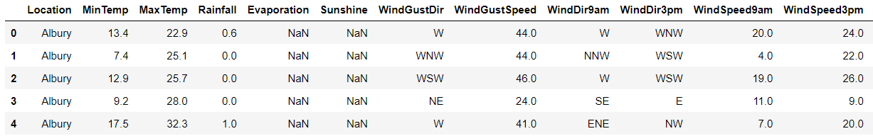
Dataset can be loaded using a method read_csv().

# Checking the Dimensions of Dataset: 

The shape property is used to find the dimensions of the dataset. 

print(rain.shape)

4. Data Preprocessing:

Real-world data is often messy, incomplete, unstructured, inconsistent, redundant, sprinkled with wacky values. So, without deploying any Data Preprocessing techniques, it is almost impossible to gain insights from raw data.

# What exactly is Data Preprocessing?

Data preprocessing is a process of converting raw data to a suitable format to extract insights. It is the first and foremost step in the Data Science life cycle. Data Preprocessing makes sure that data is clean, organize and read-to-feed to the Machine Learning model.

# A concise summary of a Dataset:

print(rain.info())

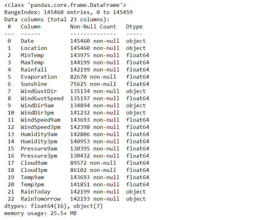
• Dataset has two data types: float64, object
• Except for the Date, Location columns, every column has missing values.

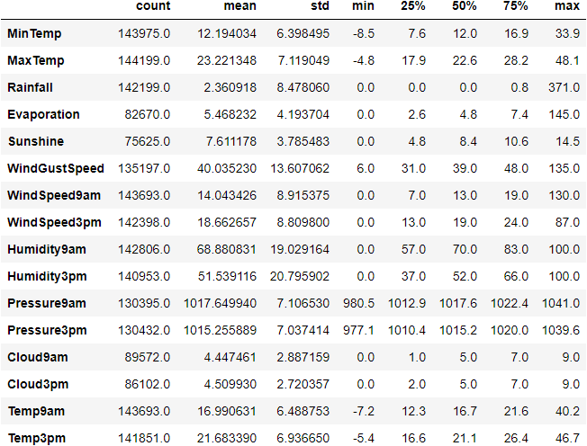
Let’s generate descriptive statistics for the dataset using the function describe() in pandas.

Descriptive Statistics: It is used to summarize and describe the features of data in a meaningful way to extract insights. It uses two types of statistic to describe or summarize data:

• Measures of tendency
• Measures of spread

print(rain.describe(exclude=[object]))

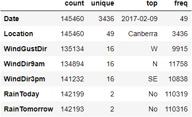
print(rain.describe(include=[object]))

5. Finding Categorical and Numerical Features in a Data set:

# Categorical features in Dataset:

categorical_features = [column_name for column_name in rain.columns if rain[column_name].dtype == 'O']
print("Number of Categorical Features: {}".format(len(categorical_features)))
print("Categorical Features: ",categorical_features)

# Numerical Features in Dataset:

numerical_features = [column_name for column_name in rain.columns if rain[column_name].dtype != 'O']
print("Number of Numerical Features: {}".format(len(numerical_features)))
print("Numerical Features: ",numerical_features)

6. Cardinality check for Categorical features:

• The accuracy, performance of a classifier not only depends on the model that we use, but also depends on how we preprocess data, and what kind of data you’re feeding to the classifier to learn.
• Many Machine learning algorithms like Linear Regression, Logistic Regression, k-nearest neighbors, etc. can handle only numerical data, so encoding categorical data to numeric becomes a necessary step.  But before jumping into encoding, check the cardinality of each categorical feature.
• Cardinality: The number of unique values in each categorical feature is known as cardinality.
• A feature with a high number of distinct/ unique values is a high cardinality feature. A categorical feature with hundreds of zip codes is the best example of a high cardinality feature.
• This high cardinality feature poses many serious problems like it will increase the number of dimensions of data when that feature is encoded. This is not good for the model.
• There are many ways to handle high cardinality, one would be feature engineering and the other is simply dropping that feature if it doesn’t add any value to the model.

Let’s find the cardinality for Categorical features:

for each_feature in categorical_features:
   unique_values = len(rain[each_feature].unique())
   print("Cardinality(no. of unique values) of {} are: {}".format(each_feature, unique_values))

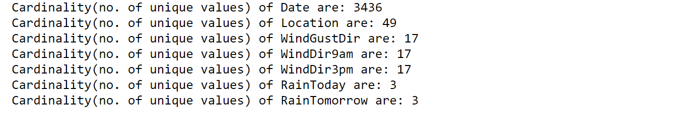
Date column has high cardinality which poses several problems to the model in terms of efficiency and also dimensions of data increase when encoded to numerical data.

# Feature Engineering of Date column to decrease high cardinality:

rain['Date'] = pd.to_datetime(rain['Date'])
rain['year'] = rain['Date'].dt.year
rain['month'] = rain['Date'].dt.month
rain['day'] = rain['Date'].dt.day

Drop Date column:

rain.drop('Date', axis = 1, inplace = True)
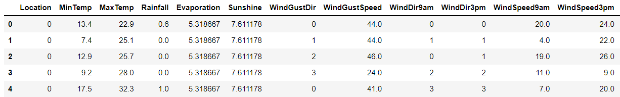
rain.head()

7. Handling Missing Values:

Machine learning algorithms can’t handle missing values and cause problems. So they need to be addressed in the first place. There are many techniques to identify and impute missing values.

If a dataset contains missing values and loaded using pandas, then missing values get replaced with NaN(Not a Number) values. These NaN values can be identified using methods like isna() or isnull() and they can be imputed using fillna(). This process is known as Missing Data Imputation.

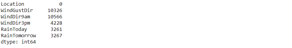
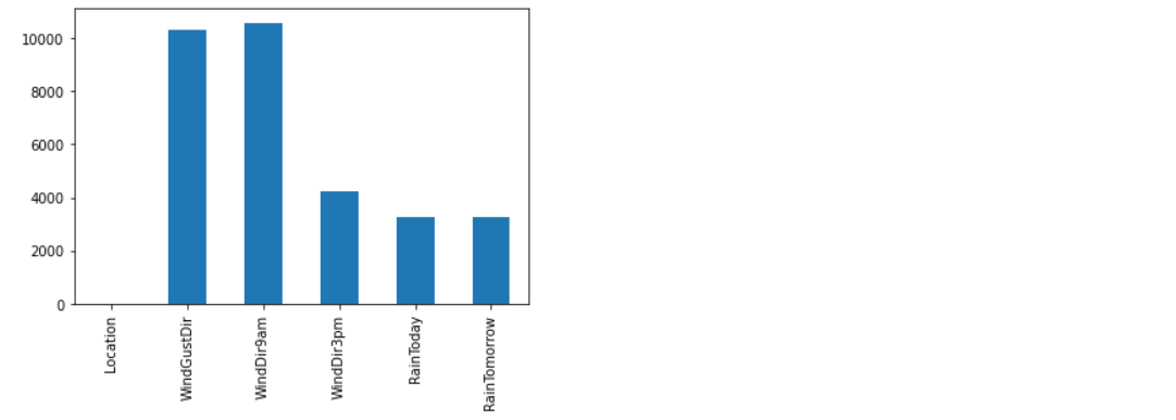
# Handling Missing values in Categorical Features:

categorical_features = [column_name for column_name in rain.columns if rain[column_name].dtype == 'O']
rain[categorical_features].isnull().sum()

# Imputing the missing values in categorical features using the most frequent value which is mode:

categorical_features_with_null = [feature for feature in categorical_features if rain[feature].isnull().sum()]
for each_feature in categorical_features_with_null:
    mode_val = rain[each_feature].mode()[0]
    rain[each_feature].fillna(mode_val,inplace=True)

# Handling Missing values in Numerical features:

numerical_features = [column_name for column_name in rain.columns if rain[column_name].dtype != 'O']
rain[numerical_features].isnull().sum()

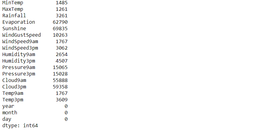
Missing values in Numerical Features can be imputed using Mean and Median. Mean is sensitive to outliers and median is immune to outliers. If you want to impute the missing values with mean values, then outliers in numerical features need to be addressed properly.

8. Outliers detection and treatment:

# What is an outlier?

An Outlier is an observation that lies an abnormal distance from other values in a given sample. They can be detected using visualization(like boxplots, scatter plots), Z-score, statistical and probabilistic algorithms, etc.

# Outlier Treatment to remove outliers from Numerical Features:

features_with_outliers = ['MinTemp', 'MaxTemp', 'Rainfall', 'Evaporation', 'WindGustSpeed','WindSpeed9am', 'WindSpeed3pm', 'Humidity9am', 'Pressure9am', 'Pressure3pm', 'Temp9am', 'Temp3pm']
for feature in features_with_outliers:
    q1 = rain[feature].quantile(0.25)
    q3 = rain[feature].quantile(0.75)
    IQR = q3-q1
    lower_limit = q1 - (IQR*1.5)
    upper_limit = q3 + (IQR*1.5)
    rain.loc[rain[feature]<lower_limit,feature] = lower_limit
    rain.loc[rain[feature]>upper_limit,feature] = upper_limit

Now, numerical features are free from outliers. Let’s Impute missing values in numerical features using mean.

numerical_features_with_null = [feature for feature in numerical_features if rain[feature].isnull().sum()]
for feature in numerical_features_with_null:
    mean_value = rain[feature].mean()
    rain[feature].fillna(mean_value,inplace=True)

It’s time to do some analysis on each feature to understand about data and get some insights.

9. Exploratory Data Analysis:

Exploratory Data Analysis(EDA) is a technique used to analyze, visualize, investigate, interpret, discover and summarize data. It helps Data Scientists to extract trends, patterns, and relationships in data.

1. Univariate Analysis:

a) Exploring target variable:

rain['RainTomorrow'].value_counts().plot(kind='bar')

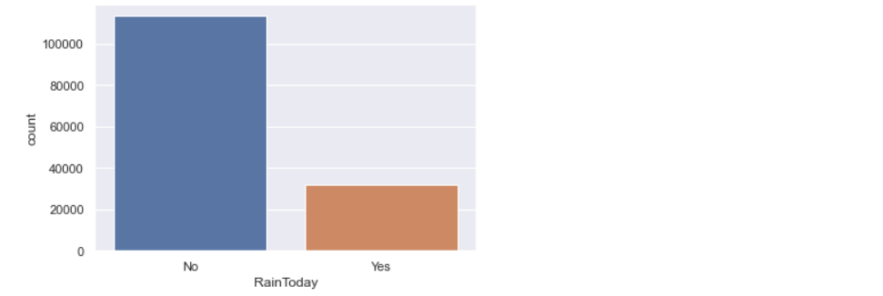
Looks like the Target variable is imbalanced. It has more ‘No’ values. If data is imbalanced, then it might decrease the performance of the model. As this data is released by the meteorological department of Australia, it doesn’t make any sense when we try to balance the target variable, because the truthfulness of data might decrease. So, let me keep it as it is.

2. Bi-variate Analysis:

a) Sunshine vs Rainfall:

sns.lineplot(data=rain,x='Sunshine',y='Rainfall',color='green')

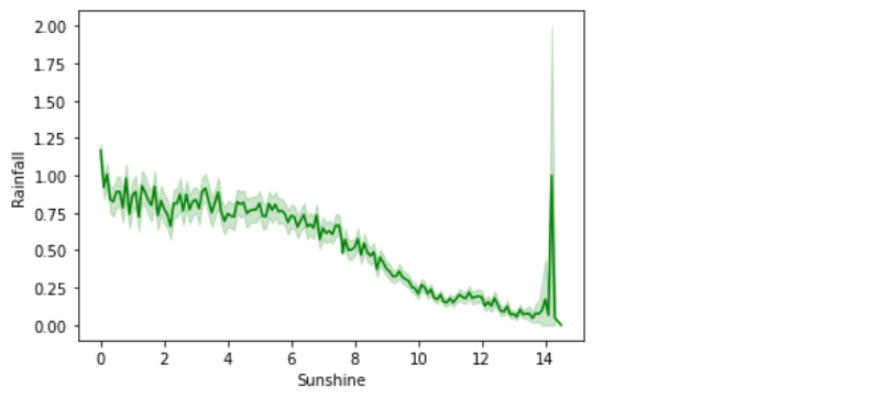
In the above line plot, the Sunshine feature is inversely proportional to the Rainfall feature.

b) Sunshine vs Evaporation:

sns.lineplot(data=rain,x='Sunshine',y='Evaporation',color='blue')

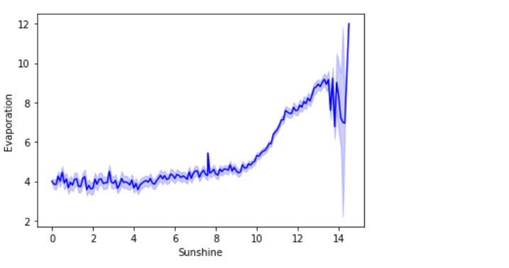
In the above line plot, the Sunshine feature is proportional to the Evaporation feature.

10. Encoding of Categorical Features:

Most Machine Learning Algorithms like Logistic Regression, Support Vector Machines, K Nearest Neighbours, etc. can’t handle categorical data. Hence, these categorical data need to converted to numerical data for modeling, which is called  Feature Encoding.

There are many feature encoding techniques like One code encoding, label encoding. But in this particular blog, I will be using replace() function to encode categorical data to numerical data.

def encode_data(feature_name):

    ''' 

    This function takes feature name as a parameter and returns mapping dictionary to replace(or map) categorical data with numerical data.

    '''

    mapping_dict = {}

    unique_values = list(rain[feature_name].unique())

    for idx in range(len(unique_values)):

        mapping_dict[unique_values[idx]] = idx

    return mapping_dict




rain['RainToday'].replace({'No':0, 'Yes': 1}, inplace = True)

rain['RainTomorrow'].replace({'No':0, 'Yes': 1}, inplace = True)

rain['WindGustDir'].replace(encode_data('WindGustDir'),inplace = True)

rain['WindDir9am'].replace(encode_data('WindDir9am'),inplace = True)

rain['WindDir3pm'].replace(encode_data('WindDir3pm'),inplace = True)

rain['Location'].replace(encode_data('Location'), inplace = True)

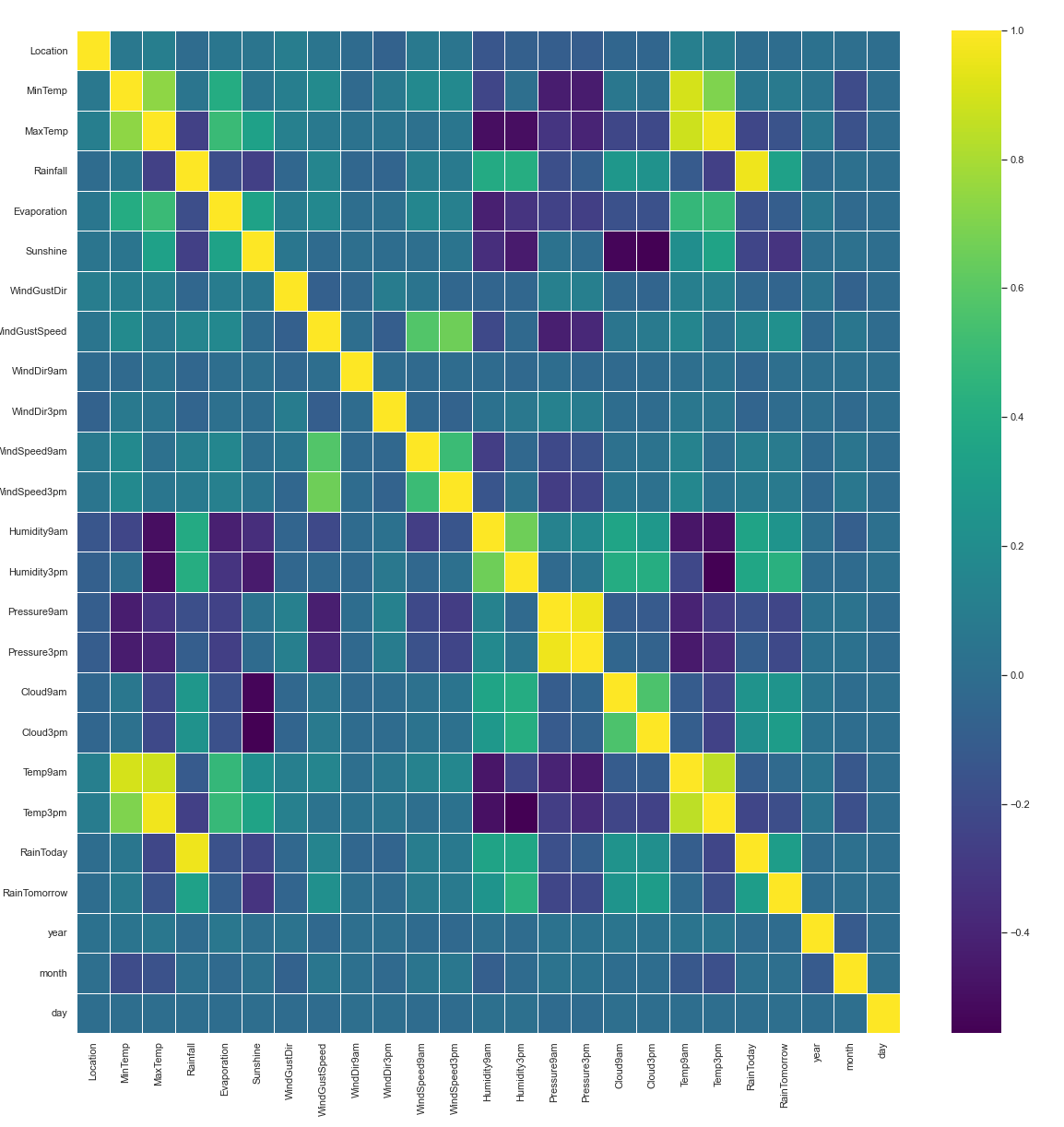
11. Correlation: 

Correlation is a statistic that helps to measure the strength of the relationship between two features. It is used in bivariate analysis. Correlation can be calculated with method corr() in pandas.

plt.figure(figsize=(20,20))
sns.heatmap(rain.corr(), linewidths=0.5, annot=False, fmt=".2f", cmap = 'viridis')

# Splitting data into Independent Features and Dependent Features:

For feature importance and feature scaling, we need to split data into independent and dependent features.

X = rain.drop(['RainTomorrow'],axis=1)
y = rain['RainTomorrow']

In the above code,

• X – Independent Features or Input features
• y – Dependent Features or target label

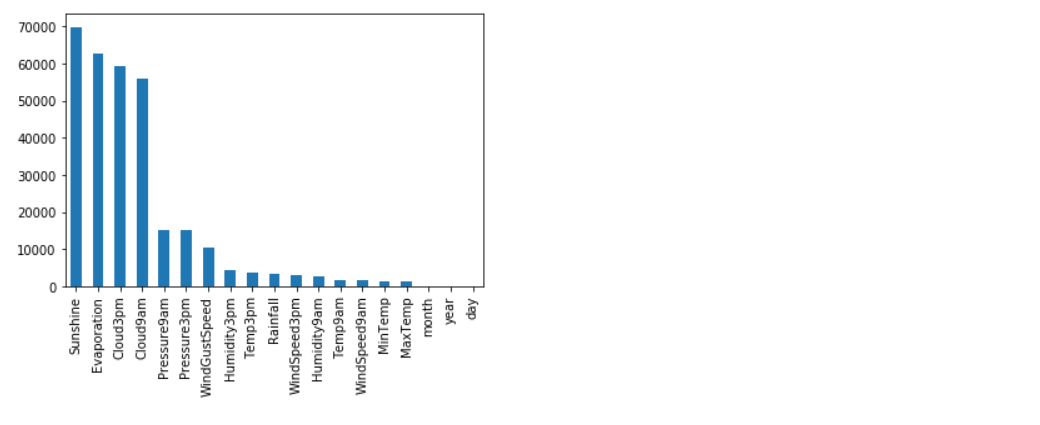
12. Feature Importance:

• Machine Learning Model performance depends on features that are used to train a model. Feature importance describes which features are relevant to build a model.
• Feature Importance refers to the techniques that assign a score to input/label features based on how useful they are at predicting a target variable. Feature importance helps in Feature Selection.

We’ll be using ExtraTreesRegressor class for Feature Importance. This class implements a meta estimator that fits a number of randomized decision trees on various samples of the dataset and uses averaging to improve the predictive accuracy and control over-fitting.

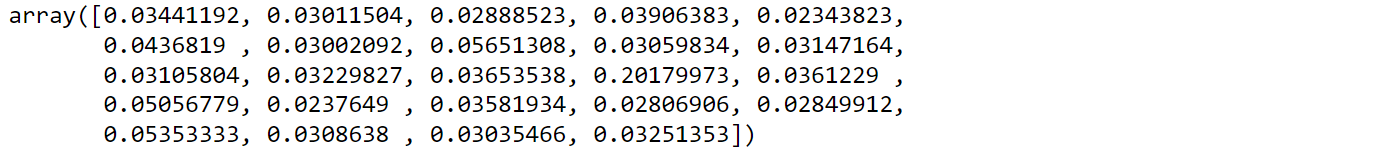
from sklearn.ensemble import ExtraTreesRegressor
etr_model = ExtraTreesRegressor()
etr_model.fit(X,y)
etr_model.feature_importances_

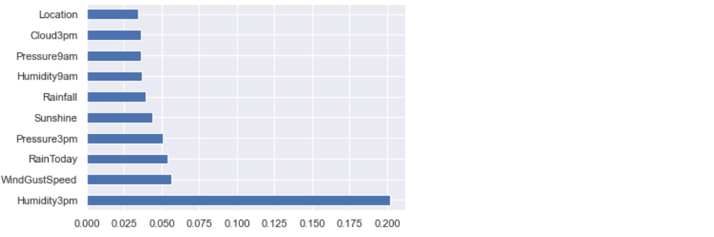
Let’s visualize feature importance values:

feature_imp = pd.Series(etr_model.feature_importances_,index=X.columns)
feature_imp.nlargest(10).plot(kind='barh')

13. Splitting Data into training and testing set:

train_test_split() is a method of model_selection class used to split data into training and testing sets.

from sklearn.model_selection import train_test_split
X_train, X_test, y_train, y_test = train_test_split(X,y, test_size = 0.2, random_state = 0)

Length of Training and Testing set:

print("Length of Training Data: {}".format(len(X_train)))
print("Length of Testing Data: {}".format(len(X_test)))

14. Feature Scaling:

Feature Scaling is a technique used to scale, normalize, standardize data in range(0,1). When each column of a dataset has distinct values, then it helps to scale data of each column to a common level. StandardScaler is a class used to implement feature scaling.

from sklearn.preprocessing import StandardScaler
scaler = StandardScaler()
X_train = scaler.fit_transform(X_train)

X_test = scaler.transform(X_test)

15. Model Building:

In this article, I will be using a Logistic Regression algorithm to build a predictive model to predict whether or not it will rain tomorrow in Australia.

• Logistic Regression: It is a statistic-based algorithm used in classification problems. It allows us to predict the probability of an input belongs to a certain category.
• It uses the logit function or sigmoid function as a core.
• According to the Data science community, logistic regression can solve 60% of existing classification problems.

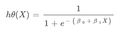
Image: Hypothesis function for Logistic Regression

# Model Training:

Sklearn library has a module called linear_model, which provides LogisticRegression class to train a model or a classifier and test it.

from sklearn.linear_model import LogisticRegression
classifier_logreg = LogisticRegression(solver='liblinear', random_state=0)
classifier_logreg.fit(X_train, y_train)

# Model Testing:

y_pred = classifier_logreg.predict(X_test)
y_pred

# Evaluating Model Performance:

accuracy_score() is a method used to calculate the accuracy of a model prediction on unseen data.

from sklearn.metrics import accuracy_score
print("Accuracy Score: {}".format(accuracy_score(y_test,y_pred)))

# Checking for Underfitting and Overfitting:

print("Train Data Score: {}".format(classifier_logreg.score(X_train, y_train)))
print("Test Data Score: {}".format(classifier_logreg.score(X_test, y_test)))

The accuracy Score of training and testing data is comparable and almost equal. So, there is no question of underfitting and overfitting. And the model is generalizing well for new unseen data.

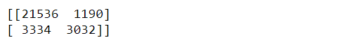
# Confusion Matrix:

A Confusion Matrix is used to summarize the performance of the classification problem. It gives a holistic view of how well the model is performing.

print(confusion_matrix(y_test,y_pred))

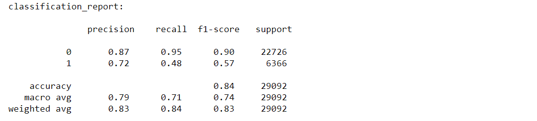
# Classification-report:

The classification report displays the values of precision, recall, F1 for the model.

 

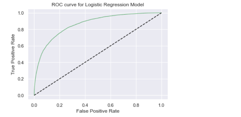
# Receiver operating characteristic(ROC) curve:

• The ROC curve is an evaluation metric used in binary classification problems to know the performance of the classifier.
• It is a curve plotted between True Positive Rate(TPR) and False Positive Rate(FPR) at various thresholds.
• ROC graph summarizes all the confusion matrices produced at different threshold values.
• ROC curve is used to determine which threshold value is best for Logistic Regression in order to classify classes.

y_pred_logreg_proba = classifier_logreg.predict_proba(X_test)
from sklearn.metrics import roc_curve
fpr, tpr, thresholds = roc_curve(y_test, y_pred_logreg_proba[:,1])
plt.figure(figsize=(6,4))
plt.plot(fpr,tpr,'-g',linewidth=1)
plt.plot([0,1], [0,1], 'k--' )
plt.title('ROC curve for Logistic Regression Model')
plt.xlabel("False Positive Rate")
plt.ylabel('True Positive Rate')
plt.show()

# Cross-Validation:

Let’s find out whether model performance can be improved using Cross-Validation Score.

from sklearn.model_selection import cross_val_score
scores = cross_val_score(classifier_logreg, X_train, y_train, cv = 5, scoring='accuracy')
print('Cross-validation scores:{}'.format(scores))
print('Average cross-validation score: {}'.format(scores.mean()))

The mean accuracy score of cross-validation is almost the same as the original model accuracy score which is 0.8445. So, the accuracy of the model may not be improved using Cross-validation.

16. Results and Conclusion:

Source: Canva

• The logistic Regression model accuracy score is 0.84. The model does a very good job of predicting.
• The model shows no sign of Underfitting or Overfitting. This means the model generalizing well for unseen data.
• The mean accuracy score of cross-validation is almost the same as the original model accuracy score. So, the accuracy of the model may not be improved using Cross-validation.

17. Save Model and Scaling object with Pickle:

Pickle is a python module used to serialize and deserialize objects. It is a standard way to store models in machine learning so that they can be used anytime for prediction by unpickling.

Here scaling object is stored in a pickle file, which can be used to standardize real-time and unseen data fed by users for prediction.

import pickle

with open('scaler.pkl', 'wb') as file:

    pickle.dump(scaler, file) # here scaler is an object of StandardScaler class.

Save the logistic regression model in a pickle file, so that it can be used for predictions later.

with open('logreg.pkl', 'wb') as file:
    pickle.dump(classifier_logreg, file) # here classifier_logreg is trained model

You can find code on my Github.

Part-2 of this article: Deployment of Model on Heroku Server using Flask. (Link will be added soon.)

                                                       . . .

About the Author:

Hello, I’m Ajay Vardhan Reddy, pursuing a Bachelor of Technology(B.Tech) in Computer Science and Engineering from Vignana Bharathi Institute of Technology, Hyderabad. I’m a Co-founder of the Machine Learning Forum, EpsilonPi. I’m a tech Enthusiast and an aspiring Machine Learning Engineer, a Data Detective. I run a tech page on Instagram.

You can connect me:

• LinkedIn
• Instagram
• Github

Thank you folks for reading. Happy Learning!

References:

ExtraTreesRegressor – Scikitlearn

Ajay Vardhan Reddy 19 Apr 2023