Auto Encoders -An Introductory Guide For Data Science Beginners

This article was published as a part of the Data Science Blogathon

Objective

This article’s main aim is to generate the images using Auto-encoder and understand its concepts, applications, and Limitations. For coding the Iris flower data-set was taken, which is a freely available and good source for beginners for learning machine learning, it comprises five attributes of 150 records which is name as petal length, petal width, sepal length, sepal width and species.

What is Auto-encoder?

An auto-encoder network is a couple of two associated networks, an encoder, and a decoder. In other words, It fundamentally contains two sections: the first is an encoder which is like the convolution neural organization except for the last layer. The point of the encoder is to take in productive information encoding from the data set and pass it as anything but a bottleneck design. The other piece of the auto-encoder is a decoder that utilizes dormant space in the bottleneck layer to recover the pictures like the data set. These outcomes backpropagate from the neural organization as the misfortune work. For example, the handwritten image of the digit is first transferred into hidden lower dimensional latent representation and then decode the hidden representation back into the image.

Typically they are limited in manners that permit them to duplicate just around and to duplicate just information that looks like the preparation information. Since the model is compelled to focus on which parts of the information ought to be duplicated, it frequently learns valuable properties of the information.

Encoder

Let’s understand encoder in detail, it is a neural network that takes data x which has output z along with weight and biases; for example, let’s take the value of data x as 28 i.e by 28-pixel of handwritten number, the encoder encodes it into hidden space z, with less than 784 dimensions which are also called as a bottleneck, its output parameter is qθ​(z∣x), which is nothing but a Gaussian probability density.

Decoder

Decoder, is just opposite of encoder, its input data is z, consists of weight and biases. It is represented as pϕ(x∣z).

For example, let’s consider each picture of black and white represents 0 or 1 pixel. Each pixel probability distribution can be represented by the Bernouli distribution. It takes input z and output 784 which is Bernoulli parameters.

The drawback is information from the original vector cannot be transmitted, and the reason is information is stored in less than a 784-dimensional vector.

Now the question arises of how we calculate the information which is lost and how much quantity is calculated by log-likelihood logp ϕ (x∣z).

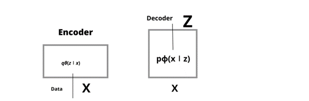
                                        Fig1  Architecture of Encoder and Decoder

 Applications

1. Dimensional Reduction and PCA when we use under-complete auto-encoders, we acquire the inert code space, whose measurement is not related to the data. It is data used as input. Additionally, utilizing a straight layer with mean-squared blunder likewise permits the organization to function as PCA.

2. Denoising auto-encoders could be used for the reasons for picture denoising. Auto-encoders can likewise be utilized for picture pressure somewhat. More on this in the limits part.

Limitations

It is used for the recreation of images, but images produced are not efficient enough when dealing with compressed images.

Another restriction is that the inert space vectors are not consistent. This implies that we can often imitate the yield pictures to include pictures. Yet, we can’t produce new images from the inert space vector. This is the place where Variational auto-encoders work superior to standard auto-encoders.

Code-

import warnings
warnings.filterwarnings('ignore')
import numpy as np
import matplotlib.pyplot as plt
from scipy.stats import norm
import tensorflow as tf
from tensorflow.keras.layers import Input, Dense, Lambda
from tensorflow.keras.models import Model
from tensorflow.keras import backend as K
from tensorflow.keras import metrics

The first step involves importing the libraries NumPy, matplotlib, TensorFlow, scipy, etc.

import pandas as pd
iris = pd.read_csv("Iris.csv")
iris.head(5)

Fig 2 Here Iris data-set comprises of  five columns which include ID, Sepal Length Cm, Sepal WidthCm, Petal LengthCm, Petal WidthCm

Let’s now divide the data into train and test data.

import numpy as np 
train_set, test_set= np.split(iris, [int(.50 *len(iris))])

train_set.shape

output- (75,5)

test_set.shape

output- (75,5)

Let’s now convert the train and test data into float

x_train = np.array(train_set).astype('float32') / 255.

x_test = np.array(test_set).astype('float32') / 255.

We will now use Autoencoder

from sklearn.metrics import accuracy_score, precision_score, recall_score

from sklearn.model_selection import train_test_split

from tensorflow.keras import layers, losses

from tensorflow.keras.datasets import fashion_mnist
from tensorflow.keras.models import Model
latent_dim = 64 
class Autoencoder(Model):
  def __init__(self, latent_dim):
    super(Autoencoder, self).__init__()
    self.latent_dim = latent_dim   
    self.encoder = tf.keras.Sequential([
      layers.Flatten(),
      layers.Dense(latent_dim, activation='relu'),
    ])
    self.decoder = tf.keras.Sequential([
      layers.Dense(5, activation='sigmoid'),
      
    ])
  def call(self, x):
    encoded = self.encoder(x)
    decoded = self.decoder(encoded)
    return decoded


autoencoder = Autoencoder(latent_dim)


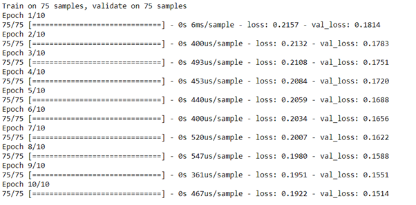
autoencoder.fit(x_train, x_train,
                epochs=10,
                shuffle=True,
                validation_data=(x_test, x_test))

autoencoder.compile(optimizer=’adam’, loss=losses.MeanSquaredError())

encoded_imgs = autoencoder.encoder(x_test).numpy()
decoded_imgs = autoencoder.decoder(encoded_imgs).numpy()

Now we are going to plot the encoded and decoded image of Iris dataset.

from matplotlib.pyplot import figure

n = 3

plt.figure(figsize=(20, 8))

for i in range(n):

  # display original

  ax = plt.subplot(2, n, i + 1)

  plt.title('original')

  lum_img = encoded_imgs[:, :, ]

  plt.imshow(lum_img, cmap="hot")

  # display reconstruction

  ax = plt.subplot(2, n, i + 1 + n)

  lum_img = decoded_imgs[:, :, ]

  plt.imshow(lum_img, cmap="hot")

  plt.title("reconstructed")

plt.show()

Fig 2 Here shows the encoded and decoded image of the Iris data set.

We have used a Matplotlib colour plot to produce the image.

Sonia Singla 11 Jul 2021