Geometrical Approach To Understand Logistic Regression

This article was published as a part of the Data Science Blogathon

Introduction

Logistic Regression is another statistical model which is used for binary classification. It’s named “Regression” because the underlying technology is similar to “Linear Regression”.

Here in this article, we will discuss:

• Understanding the Basics(Logistic Regression).

• Formulating the equation(finding better Hyperplane).

• The solution to the Outlier Problem(Sigmoid).

• Usage of Monotonic Function(log).

• Need of Regularization(Lambda).

• Getting started with the Code(Logistic Regression vs SGD with log loss).

Understanding the Basics

Let’s say we have a problem with spam emails and we want to keep the Non-spam(Ham) in the Inbox and send the Spam to the Spam folder

Fig 1:Spam and Non-Spam email

We have two types of email Spam and Ham, let’s look at the different features of spam email. The spam email contains

• Unfriendly domain names

• The number of appearances of words “loan”,” amount”

• Spelling mistakes

There will be lots of other features but for now, let’s stick with these.

If we plot the number of times the word “loan” appears on the email on the x-axis and the spelling mistakes on the y-axis we get a pretty decent graph where the Spam and Ham can be separated using a line. And this is what logistic regression is. Basically, we want data that is linearly separable into two classes.

e.g. Here we want to separate Ham and Spam, for this, we need good features which help us in the classification.

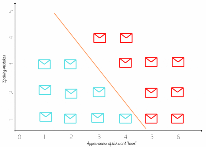
Fig 2:Plot of two features

Formulating the equation

Now if the data(i.e. all emails) is linearly separable then a line can separate the data points(each email) into two classes(Spam and Ham). For humans, it’s easy to plot the line in the 2D chart, but for computers, we must follow sets of instructions.

So let’s consider the Ham as positive class “+1”, Spam as negative class “-1” and we have “n” number of features.

In 2-D the equation of the line is : w₁x₁+w₂x₂+w₀=0

In 3-D the equation of the plane is : w₁x₁+w₂x₂+w₃x₃+w₀=0

In n-D the equation of the hyperplane is => w₁x₁+w₂x₂+w₃x₃+……….w_nx_n+w₀=0

=> [w₁,w₂,w₃……….w_n]^T[x₁,x₂,x₃……….x_n]+w₀=0

=> w_i^Tx_i+w₀=0

If the hyperplane passes through the origin then w0 becomes 0 then the equation becomes w_i^Tx_i=0. Now our task is to find the hyperplane that separates the data points.

Let’s construct a hyperplane and consider a normal unit vector “w” consisting of randomly selected values(w_i) for “w”. Now we want to find out how many data points have been correctly classified by this hyperplane.

For this we will take the help of the “equation of a point from the hyperplane” i.e d_i= w^Tx_i/||w|| since we are considering w as normal unit vector(||w|| =1), therefore d_i= w^Tx_i

Now if the data points are in the same direction of the normal vector then it will belong to the positive class else it belongs to the negative class.

Let’s consider

1. A positive class data point xi which is in the direction of the normal vector, then wTxi will be greater than 0 and if we multiply it with the class label y_i=+1 then y_iw^Tx_i>0

2. A negative class data point x_j which is in the opposite direction of the normal vector then w^Tx_j will be less than 0, since y_j=-1, therefore, y_jw^Tx_j>0

3. A positive class data point x_i which is in the opposite direction of the normal vector, then w^Tx_i will be less than 0 and the class label y_i=+1 then y_iw^Tx_i<0 i.e data point has been incorrectly classified.

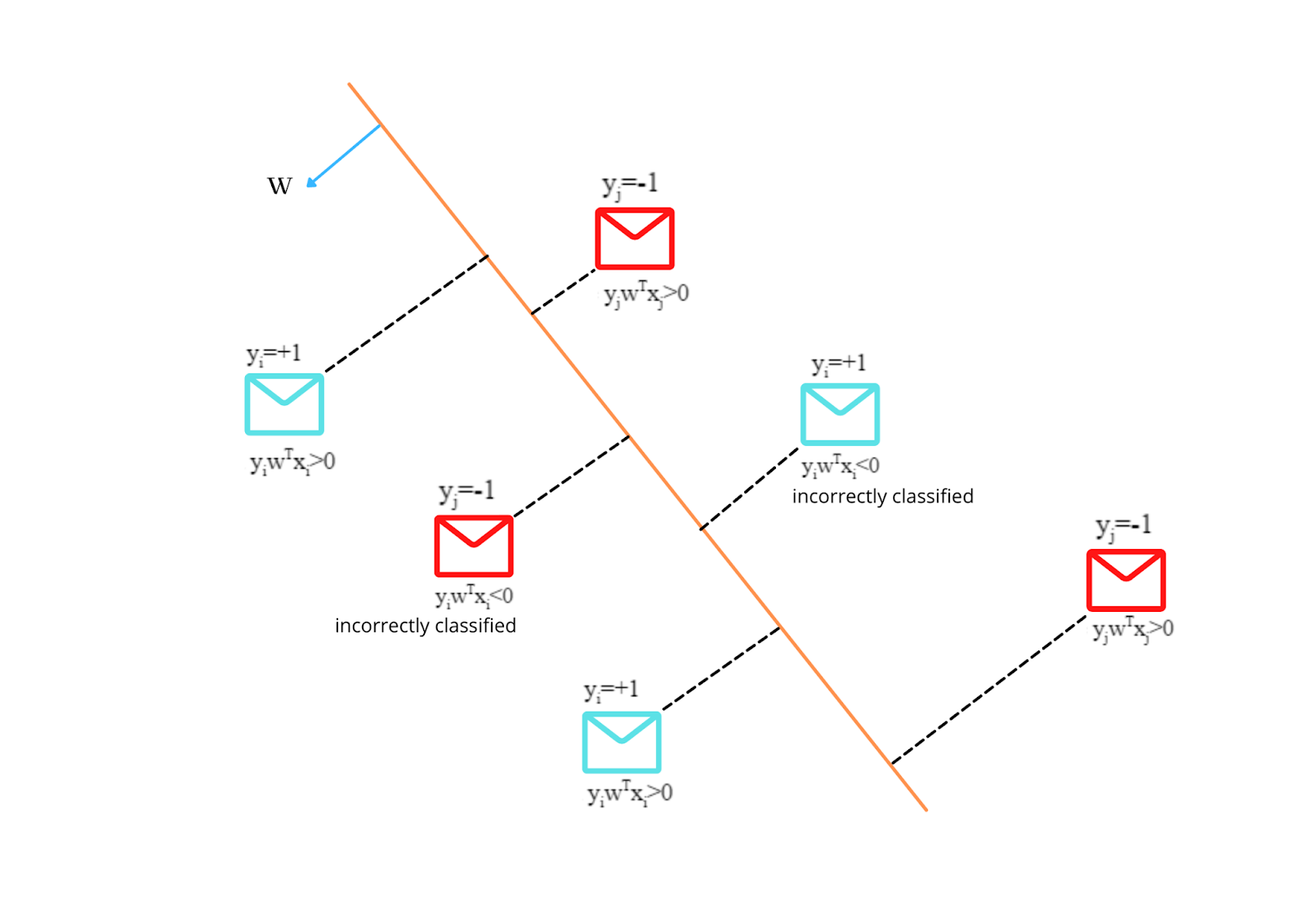
Fig 3:How hyperplane separates the data points

From the above hyperplane h₁ if we sum all the data points

Let y_iw^Tx_i=1 for correctly classified and -1 for incorrectly classified

sum(h₁) = 1+1+1+1+(-1)+(-1)

= 4

Suppose if we have another hyperplane h₂ where the sum(h₂) is equal to 5 then h₂ is a better hyperplane than h₁

So, we want the best hyperplane which minimizes the number of misclassifications and maximizes the sum.

The solution to the Outlier Problem

Now, if we have an outlier on either side of the hyperplane then it will impact the sum. Hence it will impact the selection of the best hyperplane.

For example:

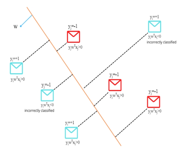
Fig 4:Outlier affecting the hyperplane

 

Even Though the hyperplane separates the data points correctly, the summation gets impacted by the outlier.

Since w^Tx_outlier >> w^Tx_{correctly_classifier} therefore, y_iw^Tx_outlier will reduce the overall sum for that hyperplane.

To deal with the outliers which impact the values of w, we will be using the sigmoid function.

Sigmoid(x)=1/(1+e^-x)

Lets us assume we have an outlier then w^Tx_outlier >> w^Tx_{correctly_classifier}

Now if we use the sigmoid function then sigmoid(w^Tx_outlier) << w^Tx_outlier

When the value of w^Tx_outlier becomes larger it tapers it off, the values of w^Tx are squashed from [-infinity,+infinity] to [0,1].

 

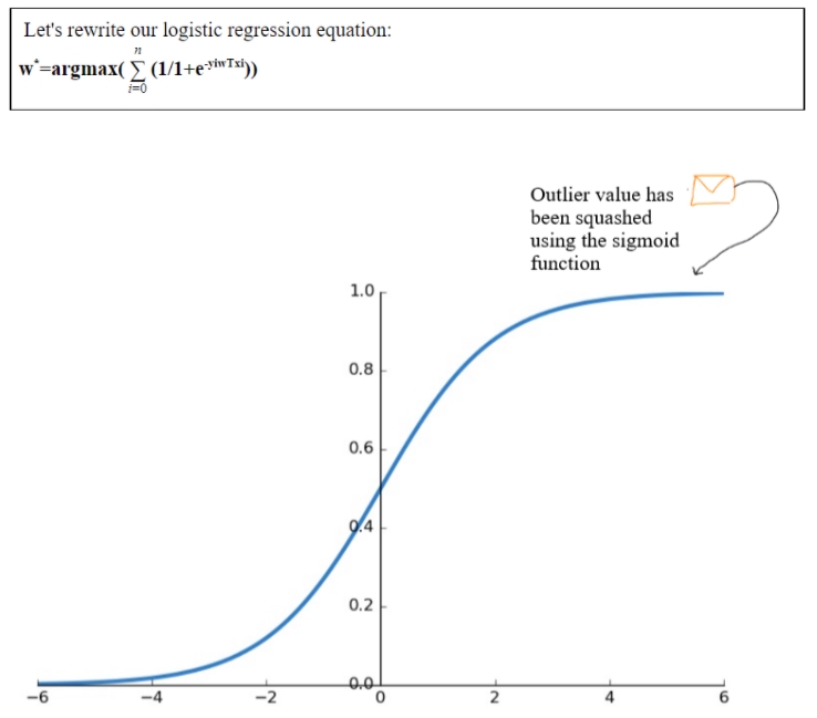
Fig 5:Sigmoid function and how it helps to reduce the value of outliers

 

Monotonic Function

We know that a monotonic function increases with increasing the value of x and if a function is monotonic then when applied a monotonic function retains the same maxima or minima i.e

• x increases then f_monotonic(x) increases                                                    (i)

• Argmin f_monotonic(x) = Argmin g_monotonic(f_monotonic(x))            (ii)

• Also we know that Argmax – f(x) = Argmin f(x)                       (iii)

• Log is also a monotonic function and log(1/x) = -log(x)       (iv)

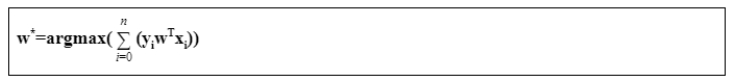
Our logistic regression equation: w*= argmax(summation_i=0_to_n(1/1+e^-yiwTxi))

Need of Regularization

We have learned how these functions are being used to understand the data and how to overcome various issues. Now let us understand one most important topic known as Bias and Variance Tradeoff.

Suppose we have a dataset contain emails. Now we have got an email for classification which contains the word “loan” multiple times. Our model directly classified it as “Spam” because it contains the word “loan”. Optimizing the logistic regression loss function, our model has learned that any email contains the word “loan” multiple times is “spam”. This is called overfitting i.e. high variance. We are trying to learn everything from our training data which causes our model to overfit.

Now using regularization significantly reduces the variance without increasing the bias. Regularization refers to the act of modifying a learning algorithm to favour “simpler” prediction rules to avoid overfitting. It modifies the loss function to penalize certain values of the weights.

Let z_i = y_iw^Tx_i

=> z_i-> + infinity, then  exp(-z_i) -> 0,

                                       Log(1+exp(-z_i)) -> 0

                                       w^* = 0

If the selected “w” classifies all the training points correctly and if z_i tends to “- infinity” then the selected “w” is the best “w” on training data. This is a condition of overfitting as the training data may contain outliers to which our model has been perfectly fitted. So, we will add the regularization to deal with the problem.

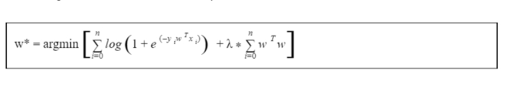
Here “lambda” is a hyperparameter.

• If lambda = 0 then the loss term optimization results in an overfitting model i.e. high variance

• If lambda is larger then the loss term diminished and this leads to an underfitting model i.e. high bias

 

Fig 6:Logistic Loss vs Regularization

The regularization term will constrain w from reaching “+infinity” and “-infinity”.

We can also use L1 regularization which induces sparsity(most of the elements of the weight vector are zero) into the weight vector. The less important features vanish in Logistic Regression with L1 Regularization while using L2 the weight for the less important features becomes small but remains non-zero.

Getting Started with the Code

Let’s understand the code of the Logistic Regression

1. 1. Using Logistic Regression, which by default uses Gradient Descent. Here “lambda” is a hyperparameter. Here “lambda” is hyperparameter C=1/lambda and as C increases it will overfit and as C decreases it will underfit.

      from sklearn.datasets import load_iris
      from sklearn.linear_model import LogisticRegression
      #Importing the Logistic Regression and iris dataset
      X, y = load_iris(return_X_y=True)
      clf = LogisticRegression(C=0.01).fit(X, y)
      #Setting the hyperparameter for the Logistic Regression and #training the model
      clf.predict(X[:2, :])
      #Predicting the class for the data point
      clf.predict_proba(X[:2, :])
      #We can also predict the probability of the class

   2. Using Stochastic Gradient Descent

By simply changing the loss parameter we can easily switch between different Classifiers. For logistic regression we will use loss=” log”, for SVM we will use “Hinge” and so on.

from sklearn.linear_model import SGDClassifier
#Importing the SGDClassifier
X = [[0., 0.], [1., 1.]]
y = [0, 1]
clf = SGDClassifier(loss="log")
#Setting the parameter loss=”log” for Logistic Regression
clf.fit(X, y)
#Training the model
clf.predict([[2., 2.]])
#Predicting the class for the data point

 

Conclusion

Logistic Regression performs well when the data is linearly separable but in the real world, the data is rarely linearly separable. It is less prone to overfitting but we should consider using regularization techniques to avoid overfitting.

Rajdeep Borgohain 23 Jul 2021