Introduction To Audio Classification -Emergency vs Nonemergency Vehicle

This article was published as a part of the Data Science Blogathon

Introduction

Audio is a series or a sequence of sounds. Every sound has a frequency and each sound can only be accessed at that particular frequency. In the realm of data science, there are many real-world situations where one needs to work with audio data. Some of the applications are audio recommendation, audio segmentation Another very prominent use case of audio data is Audio classification, which we shall explore in this article.

Audio or sound classification is the process to listen, analyze and classify audio recordings. It is widely applicable from the translation of speech to text, recognizing sounds, identification of music or songs, automatic speech recognition, and virtual assistants.

In this article, we will start with understanding the basic concepts and terminologies for audio data and audio signals. What are types of audio signals, and how to represent the audio data into the language of what the machine understands?

In the second part of this article, we shall execute and perform audio classification on a real-life problem of classifying emergency and non-emergency vehicles based on the sound in Python using Keras.

Also, given the nature of the audio and the complexities associated with it will be using deep learning algorithms such as Convolutional Neural Network(CNN) and Long-Short Term Memory (LSTM) to build the model.

In case, you are thinking why are we using CNN for audio data, then refer to this blog on CNN for Audio Classification.

Table of Contents

• Basics of Audio Data and Audio Signals
  • Amplitude
  • Cycle
  • Frequency
  • Types of Audio Signals
  • Conversion of Audio Signals
  • Ways for Audio Signals Representation

• Problem Statement and Data
• Libraries used for Audio Classification
• Data Preparation for Model 
• Playing the Audio Data
• Visualizing the Audio Data
• Audio Classification using Time Domain features
  • Model Building using CNN
  • Model Building using LSTM
• Audio Classification using Spectrogram features
  • How is the Spectrogram computed?
  • Visualizing the Spectrogram
  • Extract the spectrogram features
  • Model Building using CNN
  • Model Building using LSTM

Basics of Audio Data and Audio Signals

Any object that vibrates produces sound waves e.g. a tuning fork or even your mobile phone. These produce a characteristic sound when it vibrates. The vibrations generated produce sound.

Now, when an object vibrates, the air molecules oscillate to and fro from the resting position of the object and transmits their energy to the neighbouring and adjacent molecules. This results in the transmission of energy from one molecule to another — which in turn — produces a sound wave.

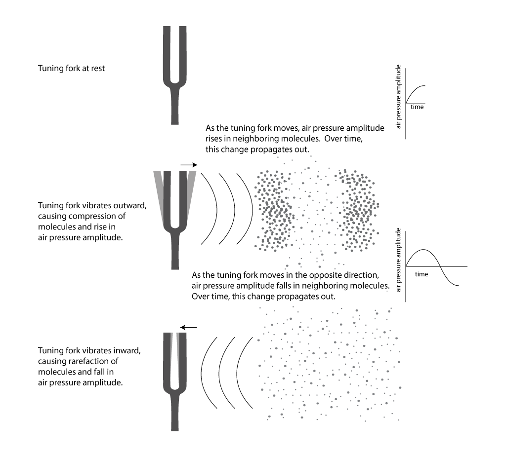
Source: digitalsoundandmusic.schwartzsound.com

This representation of sound is known as the audio signal. An audio signal has the following few important parameters, wavelength, period, amplitude, and frequency, which are very helpful in building the model and in solving the business problem:

Amplitude

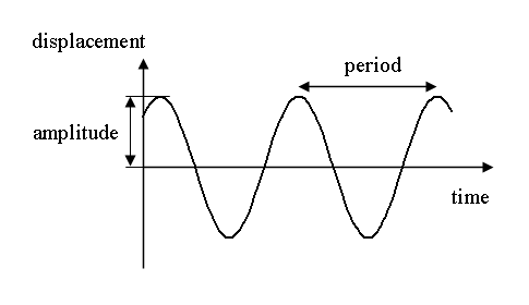
Amplitude is the maximum displacement or deviation of a particle from the rest position. At times, the rest position is also known as the mean position.

In the below image, the black horizontal line represents the equilibrium (or the mean or rest) position, and the maximum deviation from this black line is known as the amplitude.

Source: fowlerearthscience.weebly.com

In other words, amplitude tells how much a particle deviates from the equilibrium normal undisturbed position. It is the height of the crest or the depth of the trough, as depicted by the dotted lines in the above image.

Moving on to understanding how sound or audio moves …

Cycle

Audio waves travel in the form of cycles. A cycle is one complete upward and downward movement of the wave to its mean position.

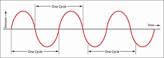
Source: techblog.ctgclean.com

Next in the line is frequency …

Frequency

Frequency refers to how fast an audio signal is changing over time. It can also be referred to as the number of cycles per second.

In other words, the number of occurrences of a repeating wave (a repeating wave is equal to the cycle) per unit of time is called frequency.

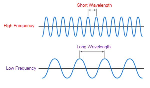
Source: techplayon.com

It is worth noting that:

• A cycle can start anywhere within an audio wave. However, it is the period of the audio wave that determines the frequency, not from where the cycle started.
• When the frequency increases twofold, then the number of waves also increases twofold at any given time.
• Low frequencies will have long-wavelength or larger periods and high frequencies will have a shorter wavelength and shorter periods.

Up until now, we saw what is an audio signal, how does it travel, and changes over time. Now let’s see what are the types in which audios are stored.

Types of Audio Signals

There are two different types of audio signals: Analog and Digital signals.

An Analog signal is a continuous wave that changes over a period of time. An infinite number of samples exists between any two consecutive time instances.

Source: thexplorion.com

On the other hand, as can see from the above image, digital signals are a discrete representation of a signal over a period of time. Here, only a finite number of values exist between any two consecutive time instances. The signals can have only one value at any point in time: either 0 or 1 i.e are binary. It can also be said that it is a discrete wave that carries information in binary form.

Conversion of Audio Signals

Now, to work on a business problem related to audio data and to process the audio signals, we would need to convert the analogue signals to digital signals. The way to do so is via Sampling.

Sampling is known as the conversion of analog signals to digital signals.

In the below image, the green color wave is the analog signal and the red points marked on it are the samples from this curve of the analog curve.

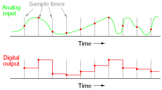
Source: ibiblio.org

How do this works is that in sampling after a fixed time interval, the value of the analog signal is measured and this sampled signal can later be used to reconstruct the original continuous signal?

Now, the average number of samples captured in one second is known as the Sampling Rate.

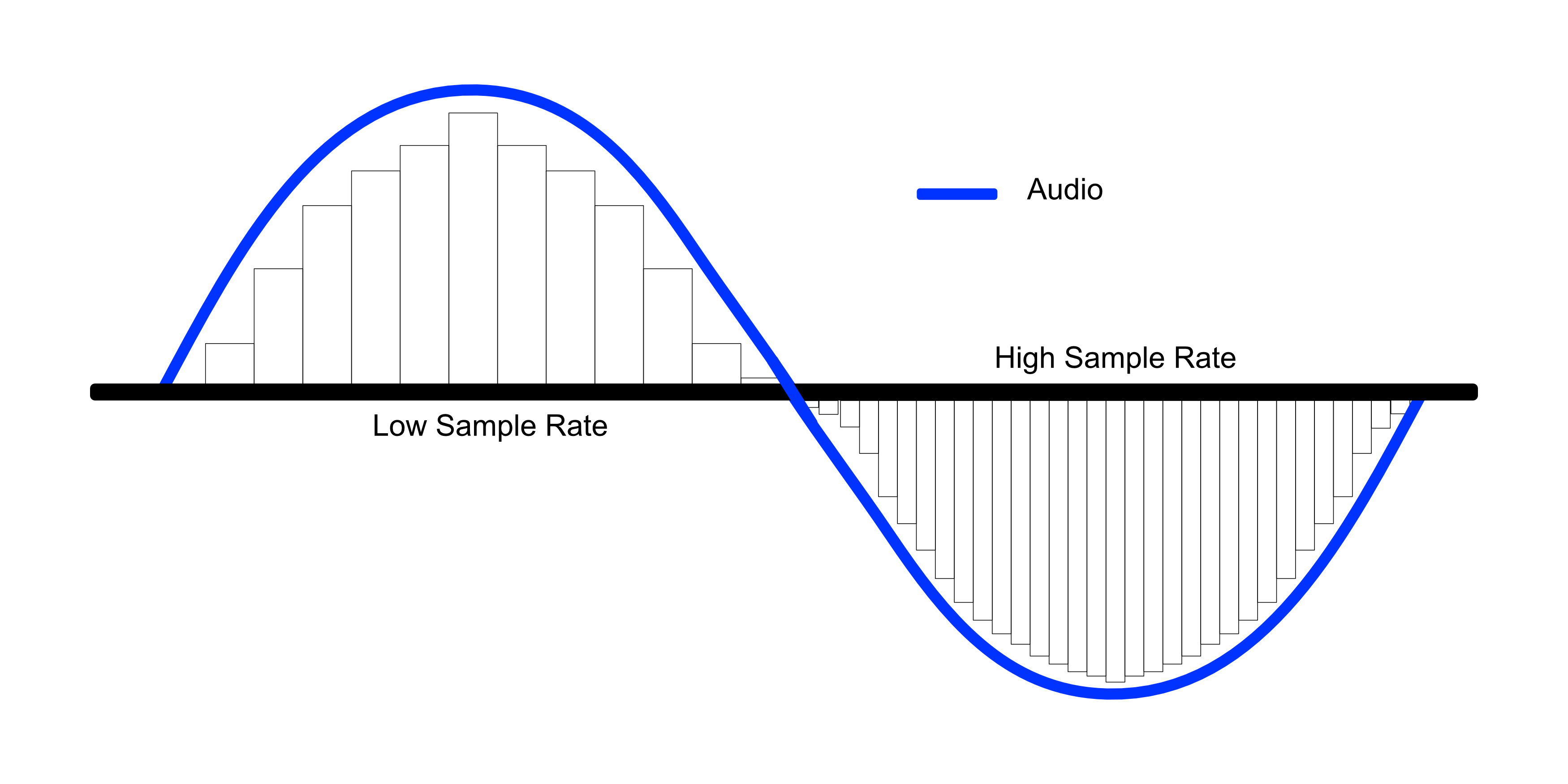
Source: cdn.shopify.com

The higher the sampling rate, the greater will be the sound quality, and also it costs more memory space.

Now, let’s move onto how are these audio signals represented.

Ways for Audio Signals Representation

There are two ways in which an audio signal can be represented via Time Domain and Spectrogram.

1. Time Domain

In the time domain, the audio is represented by the amplitude (which is represented) as a function of time i.e. amplitude is recorded at different intervals of time. In simple words, it is a plot between amplitude and time.

• X-axis: time, and
• Y-axis: amplitude
• 

Source: upload.wikimedia.org

2. Spectrogram

A spectrogram, another audio representation, is a two-dimensional (2D) plot between time and frequency having a third dimension, which exhibits colors. Each value of the spectrogram represents an amplitude of the frequency at a particular time in terms of intensity colors. This

In simple terms, it is a spectrum of frequencies as it varies with the time, where:

• The X-axis is time, where the time goes from the left (oldest) to right (youngest).
• Y-axis is frequency, where the lowest frequencies are at the bottom and the highest frequencies at the top.
• The values are the amplitudes of a particular frequency at a particular time.

Source: upload.wikimedia.org

The spectrogram is one kind of a heat map where the intensity is depicted by the varying colors and brightness. The lower color on the spectrogram represents lower intensity and lower amplitudes, and darker colors correspond to progressively stronger (or louder) amplitudes.

A spectrogram can also be seen as a visual representation of the signal strength, or the “loudness” of a signal over time at various frequencies presented in a particular waveform.

Now, we shall use the above theory to work on the case of classifying vehicles as emergency and non-emergency based on sound.

Problem Statement and Data

According to the National Crime Records Bureau, nearly 24,012 people die each day due to a delay in getting medical assistance. Many accident victims wait for help at the site, and a delay costs them their lives. The reasons could range from ambulances stuck in traffic to the fire brigade not being able to reach the site on time due to traffic jams.

The solution to the above problem is to create a system that can automatically detect the emergency vehicles before they reach the traffic signals and accordingly the traffic signals changes.

The dataset contains two .wav files: one file has emergency vehicle sounds of approximately 23 mins and another file contains sounds from non-emergency vehicles having a length of 27 mins.

The dataset and codes can be accessed from my GitHub repository.

The steps to follow are:

1. Import Libraries
2. Read the Audio Data
3. Explore and Preprocess the raw audio data
4. Split into Training and Validation Sets
5. Build Model Architecture
6. Train the Model
7. Inference

Libraries used for Audio Classification

We use the following libraries and packages in Python:

• Librosa: It is used for audio pre-processing, audio and music analysis,
  
• Scipy: It is helpful for scientific & technical computing. It contains modules for signal processing, image processing, and linear algebra. We use it here for audio features creation.
  
• Numpy: It is designed for scientific computing and data analysis. We’ll use it for array processing.
  
• IPython.display: It is used for playing the audio.
  
• Matplotib: It is used for creating two-dimensional graphs and for visualizing the data.
  
• Sklearn: This library is built upon Numpy and Scipy, comprising tools for predictive data analysis. We are using it here for splitting the data into train and test.
  
• Keras: This neural network library is used to build the model architectures, importing the respective layers, and implementing the neural nets.

After importing the required libraries, load the audio data (using load function) from the librosa library:

# importing emergency file:
emergency, sample_rate = lib.load('audio/emergency.wav', sr=16000)
# importing non-emergency file:
non_emergency, sample_rate = lib.load('audio/non emergency.wav', sr=16000)

 Finding the duration of the audio clips (using get_duration function) from the librosa library:

len1 = lib.get_duration(emergency, sr=16000)
len2 = lib.get_duration(non_emergency, sr=16000)
print('The duration of the Emergency clip is {} mins and Non-Emergency clip is {} mins.'.format(round(len1/60,2), round(len2/60,2)))

Remember, the audio waves are analogous, and to convert the sounds into the digital i.e the binary and discrete signals, the sampling process is applied. Therefore, the sample_rate (sr) of 16000 reads the above two audio clips. This sample rate means that 16000 is the average number of samples recorded per second.

Data Preparation for Model

Once the data is loaded, the next step is to prepare the audio data. As the audio files can not be directly ingested into the algorithms, hence this step of preparing the audio data is very critical.

We break the audio clip data into sequences (or chunks) of audio to train a deep learning model to perform audio classification.

How will we prepare the audio sequences?

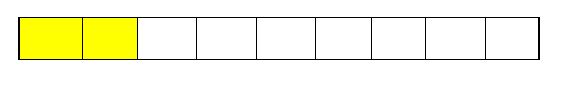
Let’s say we have a block of nine cells as shown below. In this, each cell represents one second of audio. So, we have a nine-second of audio data.

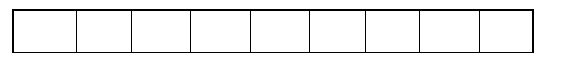
Now, we will break down this audio clip (which is of nine seconds) into audio chunks of two seconds each like this:

We get our first audio chunk (of size 2 seconds) and to extract the other audio chunks, we will slide the 2-second window one step at a time and so on.

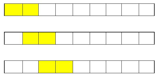
So, from the nine seconds of an audio data sequence, we will have eight audio chunks or sequences, each having a length of 2 seconds.

# User-defined Function for Audio chunks audio data is the array
def audio_chunks(audio_data, num_of_samples=32000, sr=16000):
    # empty list to store new audio chunks formed 
    data=[]
    for i in range(0, len(audio_data), sr):
        # creating the audio chunk by starting with the first second & sliding the 2-second window one step at a time 
        chunk = audio_data[i: i+ num_of_samples]
        if(len(chunk)==32000):
            data.append(chunk)
    return data

# Calling the above function audio_chunks to create seperate chunks for both Emergency and non-emergency vehicles:
emergency = audio_chunks(emergency)
non_emergency = audio_chunks(non_emergency)
print('The number of chunks of Emergency is {} and Non-Emergency is {}.'.format(len(emergency), len(non_emergency)))

We define a function in Python to break the audio data into audio chunks. Now, in our case, the sample rate for each audio file is 16000 so, the audio wave of 2 seconds with a sampling rate of 16,000 will have 32,000 samples.

After calling the function, we get the number of chunks of Emergency as 1374 and Non-Emergency as 1628.

Playing the Audio Data

Next, we will see how the audio looks by plotting amplitudes against time.

# Emergency Sound:
ipd.Audio(emergency[45], rate=16000)
# Non-Emergency Sound:
ipd.Audio(non_emergency[29], rate=16000)

The output for the above code returns a playable audio clip as below for each of the emergency and non-emergency sounds:

Visualizing the Audio Data

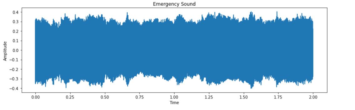
# Emergency Sound
plt.figure(figsize=(14,4))
plt.plot(np.linspace(0, 2, num=32000),emergency[32])
plt.title('Emergency Sound')
plt.xlabel('Time')
plt.ylabel('Amplitude')
plt.show()
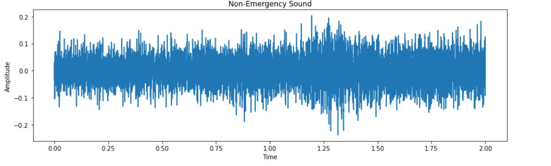
# Non-Emergency Sound
plt.figure(figsize=(14,4))
plt.plot(np.linspace(0, 2, num=32000),non_emergency[33])
plt.title('Non-Emergency Sound')
plt.xlabel('Time')
plt.ylabel('Amplitude')
plt.show()

The output for the time domain plot between amplitude and time for Emergency and Non-Emergency are:

Now, from the above-created audio chunks or sequences, we will prepare the data for training and testing. The first step is to combine the emergency and non-emergency chunks.

Here, taking the emergency sounds as label 0 and non-emergency as label 1, hence it becomes a binary audio classification problem.

# Step 1: Combining the Emergency and Non Emergency audio chunks
audio = np.concatenate([emergency,non_emergency])
# Step 2: Assigning labels 
labels1 = np.zeros(len(emergency))
labels2 = np.ones(len(non_emergency))
# concatenate labels
labels = np.concatenate([labels1,labels2])
print('The shape of the combined audio data is {}' .format(audio.shape))
# Train-test splitting:
X_train, X_test, Y_train, Y_test = train_test_split(np.array(audio), np.array(labels), stratify=labels, test_size=0.20, 
                                                    random_state=12, shuffle=True)
print('X_train', X_train.shape)
print('X_test', X_test.shape)
print('')
print('Y_train', Y_train.shape)
print('Y_test', Y_test.shape)

We have 3002 audio sequences with 32000 dimensions.

Now, a sequence model in Python expects three inputs:

• Number of samples
• Timesteps, and
• Length of the features

i.e. the input must be of a 3-dimensional array. Our input above is a 2-dimensional array hence, need to reshape the input given the requirements. As the length of the features is not present here, therefore setting the third dimension, length as 1.

# Reshaping the 2-Dimensional array into 3-Dimensional array by setting the third dimension to 1:
X_train_features = X_train.reshape(len(X_train),-1,1)
X_test_features = X_test.reshape(len(X_test), -1,1)
print('The reshaped X_train array has size:', X_train_features.shape)
print('The reshaped X_test array has size:', X_test_features.shape)

The reshaped X_train array has size: (2401, 32000, 1)
The reshaped X_test array has size: (601, 32000, 1)

The steps till now were the same whether we use time domain or spectrogram for features. Going forward, the approaches differ and we shall see all these one by one.

Audio Classification using Time Domain features

Our raw audio is already available in the time domain so, we can process it directly and start working on it. We are building the model using both CNN and LSTM. First, let’s see the steps for CNN:

Model Building using CNN

Working with the voice or audio data, we use Conv1D as it is used for input signals which are similar to the voice. Building the model with two sets of convolution and pooling layers. Defining a function comprising of the model architecture, compiler, and also the model checkpoint. This function returns two things: the model and the saved model weights.

def cnn_model(X_tr):
    inputs = Input(shape= (X_tr.shape[1], X_tr.shape[2]))
    # first Conv1D Layer with 8 filters of height 13:
    conv = Conv1D(8,13, padding='same', activation='relu')(inputs)
    conv = Dropout(0.3)(conv)
    conv = MaxPooling1D(2)(conv)
    # 2nd Conv1D Layer with 16 filters of height 11:
    conv = Conv1D(16,11, padding='same', activation='relu')(inputs)
    conv = Dropout(0.3)(conv)
    conv = MaxPooling1D(2)(conv)
    # Global MaxPooling 1D
    conv = GlobalMaxPool1D()(conv)
    # Dense Layer
    conv = Dense(16, activation='relu')(conv)
    outputs = Dense(1,activation='sigmoid')(conv)
    model = Model(inputs, outputs)
    # Model Compiler:
    model.compile(loss='binary_crossentropy', optimizer='adam', metrics =['acc'])
    # Model Checkpoint
    model_checkpoint = ModelCheckpoint('best_model_cnn.hdf5', monitor='val_loss', verbose=1, save_best_only=True, mode='min')
    return model, model_checkpoint

As it is a binary audio classification problem, therefore the loss function is binary_crossentropy.

# Calling the model:
model, model_checkpoint = cnn_model(X_train_features)
# Shape and parameters at each layer
model.summary()

Training the Model and Summarizing the history for loss:

# model training
history = model.fit(X_train_features, Y_train ,epochs=10, callbacks=[model_checkpoint], batch_size=32, 
                    validation_data=(X_test_features, Y_test))
# accuracy for the model evaluation
# load the best model weights
model.load_weights('best_model_cnn.hdf5')
# summarize history for loss
plt.plot(history.history['loss'])
plt.plot(history.history['val_loss'])
plt.title('model loss')
plt.ylabel('loss')
plt.xlabel('epoch')
plt.legend(['train', 'validation'], loc='upper left')
plt.show()

To evaluate the model performance on the test data:

# Checking the model's performance on the Test set
_, acc = model.evaluate(X_test_features, Y_test)
print("Validation Accuracy:",acc)

The model gives an accuracy of 77.038%.

Now, how do we use this model to classify the audio data into emergency vehicle sound or non-emergency vehicle sound?

To predict and classify:

# For Prediction: the input audio
index = 98
test_audio = X_test[index]
# Using IPython.display to play the audio
ipd.Audio(test_audio, rate=16000)
# classification
feature = X_test_features[index]
prob = model.predict(feature.reshape(1,-1,1))
if (prob[0][0] < 0.5):
    pred='emergency'
else:
    pred='non emergency' 
print("Prediction:",pred)

The output is an audio clip and the model predicts it as a non-emergency vehicle.

However, since the model accuracy is only 77% we can certainly improve on our model, and therefore lets’ try out another algorithm such as LSTM.

Now, building the model using the LSTM algorithm with time-domain features.

Model Building using LSTM

The shape of the input sequences is 32000. 32000 samples are meaning there will be 32000-time steps (to deal with) in every audio chunk. This can lead to a lot of time to train and the vanishing gradient descent problem can also come into place.

So, to overcome this, we’ll use a simple trick while reshaping the chunks below. Instead of keeping the length of the features (the third dimension) as 1, will use 160 which will reduce the timesteps from 32000 to just 200, and then we can easily use these reshaped sequences in our model.

# Reshaping the Audio chunks:
X_train_features = X_train.reshape(len(X_train),-1,160)
X_test_features = X_test.reshape(len(X_test), -1,160)
print('The reshaped X_train array has size:', X_train_features.shape)
print('The reshaped X_test array has size:', X_test_features.shape)

The output is:

The reshaped X_train array has size: (2401, 200, 160)
The reshaped X_test array has size: (601, 200, 160)

Building the model, in the same manner by defining user function as did for CNN:

# LSTM based deep learning model architecture
def lstm_model(X_tr):
    inputs = Input(shape=(X_tr.shape[1], X_tr.shape[2]))
    # LSTM Layer 1
    x = LSTM(128)(inputs)
    x = Dropout(0.3)(x)
    # LSTM Layer 2
    x = LSTM(128)(inputs)
    x = Dropout(0.3)(x)
    # LSTM Layer 3
    x = LSTM(64)(inputs)
    x = Dropout(0.3)(x)
    # Dense Layer
    x = Dense(64, activation = 'relu')(x)
    x = Dense(1, activation = 'sigmoid')(x)
    model = Model(inputs, x)
    # Model compiler
    model.compile(loss='binary_crossentropy', optimizer='adam', metrics=['acc'])
    # Model Checkpoint
    mc = ModelCheckpoint('best_model_lstm.hdf5', monitor='val_loss', verbose=1, save_best_only=True, mode='min')
    return model, mc

Calling the function, summary of the model:

# Calling the function
model, mc = lstm_model(X_train_features)
# Model Summary:
model.summary()

Training the model, summarizing the history loss, evaluating the model performance, and predicting for new audio data:

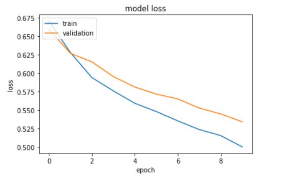
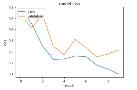
The model loss for the LSTM model built from the time-domain features is:

# Model Evaluation:
_,acc = model.evaluate(X_test_features, Y_test)
print("Accuracy:",acc)

# For Prediction using LSTM: the input audio
index = 513
test_audio = X_test[index]
# Using IPython.display to play the audio
ipd.Audio(test_audio, rate=16000)
# classification
feature = X_test_features[index]
prob = model.predict(feature.reshape(1,-1,160))
if (prob[0][0] < 0.5):
    pred='emergency vehicle'
else:
    pred='non emergency vehicle' 
print("Prediction:",pred)

The output is an audio clip and the model predicts it as a non-emergency vehicle.

We can see the validation loss decreased from 0.70 to 0.30 and the accuracy improved from 79% to 91% by using LSTM over the CNN algorithm. We had used the time domain features in both the models and going forward we will use the spectrogram features.

Audio Classification using Spectrogram features

In the case of time-domain features, the raw audio data were directly processed and started working with it. However, to work with the Spectrogram, we will:

1. First, convert the audio data into a spectrogram, and
2. then pass the spectrogram as the input array to the model

How is the Spectrogram computed?

Spectrogram accepts the raw audio wave and then breaks it into sequences or chunks and then applies fast Fourier transform (FFT) on each window to compute the frequencies.

The parameters for computing spectrogram are:

• Nperseg is the size of the window i.e. it is the number of samples in each audio chunk.
• Noverlap is the number of overlapping samples between each window. It is seen as the overlapping samples between the successive audio chunks

def spec_log(audio, sample_rate, eps = 1e-10):
    freq, times, spec = scipy.signal.spectrogram(audio, fs= sample_rate, nperseg=320, noverlap=160)
    return freq, times, np.log(spec.T.astype(np.float32) + eps)

This function scipy.signal.spectrogram returns three arrays:

1. The first array: freq: is the array of frequencies
2. The second array: times: is array segment times, and
3. The third array is spec, which is the array of the spectrogram, which is the one that is of use to us.

We are taking the log of the spectrogram because the values in the spectrogram are the amplitude values, which can be very small values of 10 to power -10 also it is hard to distinguish such small values hence, the log values.

Visualizing the Spectrogram

To visualize spectrograms two arguments are required: spectrogram and labels to distinguish.

def spec_plot(spectrogram, label):
    fig = plt.figure(figsize=(14,8))
    ax = fig.add_subplot(211)
    ax.imshow(spectrogram.T, aspect='auto', extent=[times.min(), times.max(), freqs.min(), freqs.max()])
    ax.set_title('Spectrogram of '+label)
    ax.set_xlabel('Seconds')
    ax.set_ylabel('Freqs in Hz')
    plt.show()

Calling the function to compute and visualize the spectrogram:

# Computing and Visualizing the Spectrogram for Emergency:
freqs, times, spectrogram = spec_log(emergency[162], sample_rate)
spec_plot(spectrogram,"Emergency")
# Computing and Visualizing the Spectrogram for Non-Emergency:
freqs, times, spectrogram = spec_log(non_emergency[162], sample_rate)
spec_plot(spectrogram,"Non Emergency")

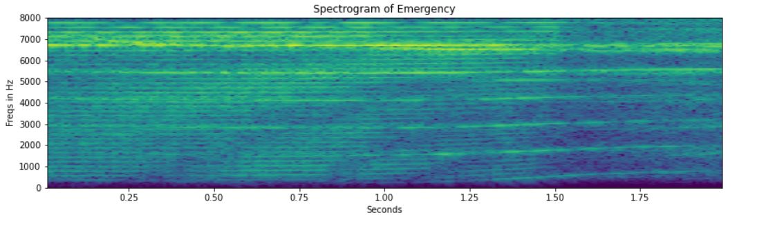
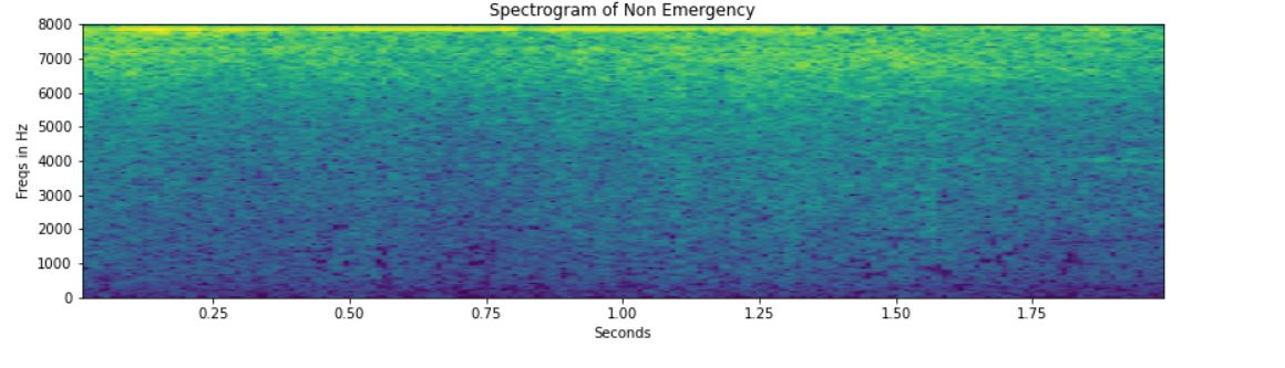
In the non-emergency vehicle’s spectrogram, no horizontal lines are depicted. This could be due to the absence of the siren sound.

Extract the spectrogram features

Extracting the spectrogram features from the same audio set that we used above during the time domain features.

def extract_spec_features(X_tr):
    # defining empty list to store the features:
    features = []
    # We only need the 3rd array of Spectrogram so assigning the first two arrays as _
    for i in X_tr:
        _,_, spectrogram = spec_log(i, sample_rate)
        mean = np.mean(spectrogram, axis=0)
        std = np.std(spectrogram, axis=0)
        spectrogram = (spectrogram - mean)/std
        features.append(spectrogram)
    # returning the features as array
    return np.array(features)
# Calling extract function to get training and testing sets:
X_train_features = extract_spec_features(X_train)
X_test_features = extract_spec_features(X_test)

These features will then be used to pass the algorithm to build the model.

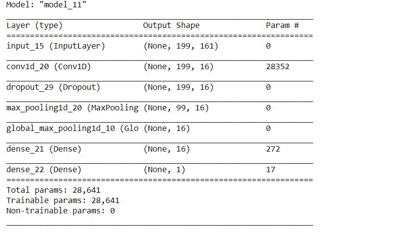
Model Building using CNN

Lets’ train the CNN-based model on the same spectrogram features using the above-defined functions for the CNN model.

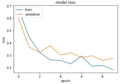
Training the model and model loss:

# Model Training:
history=model_3.fit(X_train_features, Y_train, epochs=10, callbacks=[modelcheckpoint_3], batch_size=32, 
                    validation_data=(X_test_features, Y_test))
# summarize history for loss
plt.plot(history.history['loss'])
plt.plot(history.history['val_loss'])
plt.title('model loss')
plt.ylabel('loss')
plt.xlabel('epoch')
plt.legend(['train', 'validation'], loc='upper left')
plt.show()

Evaluating the model:

# model's performance on the test set:
_,acc = model_3.evaluate(X_test_features, Y_test)
print("Accuracy:",acc)

The model returns accuracy of 97%.

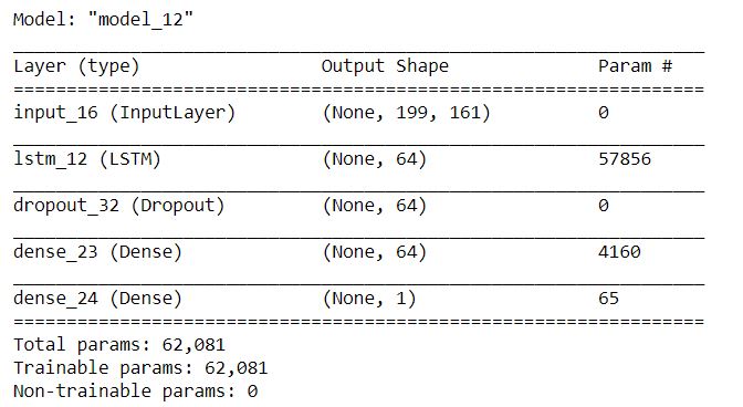
Model Building using LSTM

We can improve the accuracy further by using different algorithms, using frequency-domain features, and changing the input sequence length.

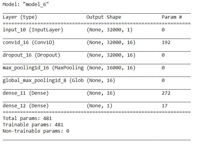
# Calling the model function
model_2, mc_2 = lstm_model(X_train_features)
# Number of parameters and shape of each layer:
model_2.summary()

 

Training the model and summarizing model loss:

# Train the model
history=model_2.fit(X_train_features, Y_train, epochs=10, callbacks=[mc_2], batch_size=32, 
                    validation_data=(X_test_features, Y_test))
model_2.load_weights('best_model_lstm.hdf5')
# summarize history for loss
plt.plot(history.history['loss'])
plt.plot(history.history['val_loss'])
plt.title('model loss')
plt.ylabel('loss')
plt.xlabel('epoch')
plt.legend(['train', 'validation'], loc='upper left')
plt.show()

Evaluating the model:

_,acc = model_2.evaluate(X_test_features, Y_test)
print("Accuracy:",acc)

The model returns an accuracy of 90.5%.

Please note: all the models are run on 10 epochs and batch size of 32 for illustrative purposes. Both the epochs and batch size are hyper-parameters. You may increase and fine-tune the model.

Endnotes

Understanding the theory and basics of audio data is very essential to solve the business problem and build the necessary model for it. The technique of how audio clips can be broken into chunks to be fed to the model is where the major task lies when it comes to working with the audio data.

I hope the articles were helpful for you to know how to work with the audio data, represent the audio data in form of both time domain and spectrogram, and eventually, build the deep learning model while working with audio data.

Thank You and Happy Learning! 🙂

About me

Hi there! I am Neha Seth, a technical writer for AnalytixLabs. I hold a Postgraduate Program in Data Science & Engineering from the Great Lakes Institute of Management and a Bachelors in Statistics. I have been featured as Top 10 Most Popular Guest Authors in 2020 on Analytics Vidhya (AV).

My area of interest lies in NLP and Deep Learning. I have also passed the CFA Program. You can reach out to me on LinkedIn and can read my other blogs for ALabs and AV.

Neha Seth 12 Jul 2021