Mathematics Behind Principle Component Analysis In Statistics

This article was published as a part of the Data Science Blogathon

Introduction

“Data is a precious thing and will last longer than the systems themselves.”

This article is based on one of the most famous dimensionality reduction techniques called PCA which stands for Principle Component Analysis. Before we discussed detailed this firstly we take a brief introduction to the dimensionality reduction concept.

let’s go…

Dimensionality Reduction

You all know that the human eye can only visualize the 1D, 2D, or 3D data easily, but what data is in the form of higher dimensions? You can visualize that N number of dimensions data with your naked eyes, for solving this problem in machine learning, we introduce dimensionality reduction. As the name suggests concept reveals that here we reduce the dimensions of the data. In simple words, we can say that dimensionality reduction is the way to transform the data of higher dimensions space to the lower dimensions space. The lower dimensions data has some meaningful information that will not affect the existence of the original data. Dimensionality reduction is common in fields that deal with large numbers of observations and/or large numbers of variables, or when we perform some machine learning fundamental tasks.

When we talk about the real world, the analysis of the data is a main task or problem for data scientists, we visualize the data by many tools and techniques, but the problem arises when we perform data analysis on the muti dimensional data, data which is 100D, 10000D and many more.

Suppose, your dataset having D-dimensions and when you want to convert it into the D-dimensions, where the D’ is less than D then this is called dimensionality reduction. What do we do then? There are several techniques for dimensionality reduction, but here we will discuss only PCA.

Principle Component Analysis

PCA is mostly using in machine learning for dimensionality reduction, PCA is the most useful dimensionality reduction technique which is used to reduce the dimensions of the data from higher to lower. By the use of this technique we extract the most useful principle component from the data but you this what is a principal component? It is simply a vector that has the variance associated with them in data.

Suppose we have an MNIST dataset, where the dataset having 784 dimensions which are very difficult to visualize we convert it into the 2-D or 3-D dimensions and then visualize it. In this article, we only get details in PCA from a visualization standpoint.

Before we move further we will discuss some key points that will generally be used in principle component analysis:

Variance: Variance is basically the spread of the data points, which means it measures how the data points. From a mathematics point of view, variance is the expectation of the squared deviation of a random variable from its mean.

Covariance:- Covariance is the method that is used to measure the relationship between two random variables or we can say how X relates to Y. Mathematically it is the summation of variance of two random variables.

Geometrical Intuition of PCA

Let’s take an example of dimensionality reduction using PCA:

Case 1:-

You know that we can’t visualize the data into higher dimensions so we take the example of 2D to 1D conversion, We reduce the 2-D data into the 1-D data.

Let’s take two features as F1 and F2 for our geometric intuition, in this F1 represents the weights of the people and another feature F2 represents the heights of the people. This represents that our dataset has 2D data F1 and F2. Now our task is to convert or reduce their dimension into 1-D

[2-D –> 1-D]

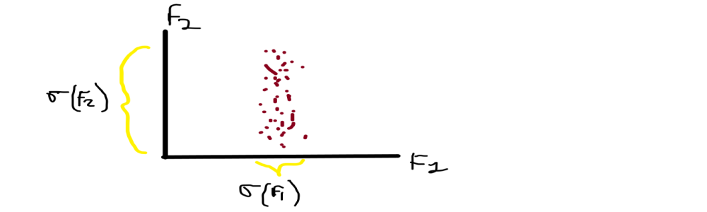
From the above image, you can see that F1 is on the x-axis and F2 is on the y-axis and having the corresponding data points Xi along with them.

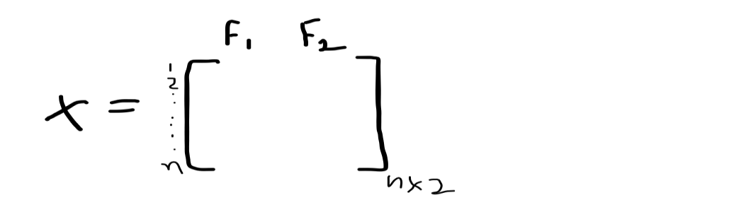
Having X data matrix which represents that we have N points and 2 features F1 and F2.

When you noticed in the graph that the data points have spread differently along with their axis, in X-axis the data is less spread means the distribution of weights are shorter ranges but if you noticed over the Y-axis the data points of height are spread very far. We recall that the variance is our spread of data, So we generally say that the variance of height is greater than the variance of weight F1( σ ) > F2( σ ).

We directed towards our main problem so we have to convert the 2D into 1D, from these 2 features we have to drop or neglect one feature for conversion, which feature do we choose? We generally pick F2 because the spread is more so the information is more. Preserving the direction with the maximum spread/variance because more spread more information.

So, our problem is solved by this we reduce the 2 dimensions to 1dimension data by picking those features whose variance is maximum.

Case 2:-

What do we do when our data is standardized? because the standardized data having an equal spread or we can say that the features that are standardized have a variance of 1 and a mean of 0 { σ =1, μ=0 }. 

mean[ F1 ] = mean[ F2 ] = 0,

variance[ F1 ] = variance[ F2 ] = 1

This is the main problem arising, what do we do now? let’s take the previous example we have to reduce 2-D to 1-D. There we pick the feature having a maximum variance, but we do some methods to solve this problem in this condition.

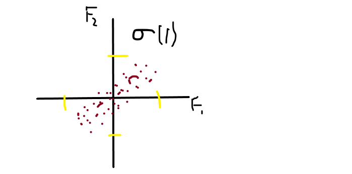
From the above image, you can see that the spread on F1 is and the spread on F2 is fairly equal because they are in the variance of 1 σ(1).

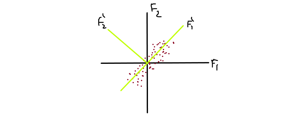
We rotate the axis with some θ angle and choose/pick that imaginary axis as our principle component, which has a maximum variance. Let’s simplify this, in the image you noticed that F1′  is the direction in which the spread is maximum and perpendicular with it we draw another axis F2′. You can see that the spread on F2′ is much much lesser than spread on F1′, represented as  [ σ( F1′ ) >> σ( F2′ ) ]. 

So, we pick F1′ because the spread is maximum and drop F2′ and we project the datapoints Xi’s into our F1′ axis.

Simplify for you that we rotate the axis in the direction where the spread or variance is maximum.

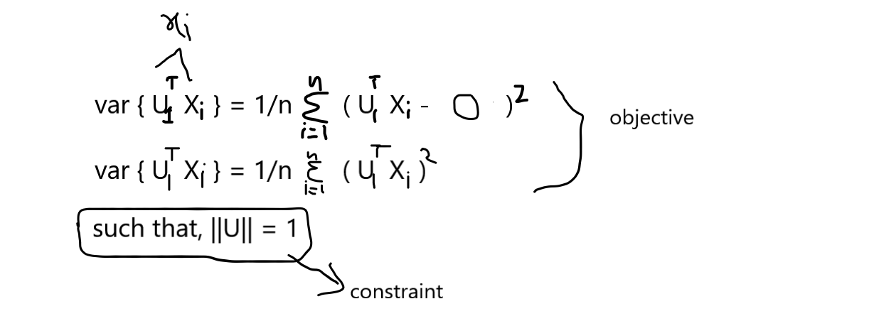
The objective of this problem is, we have to find the direction of F1′ such that the variance of Xi’s projected into F1′ is maximum.

How do we find that direction?

Once we know the direction then we project points in that direction, but how? You may know something about unit vector ||u||, if you don’t then I recall it, the unit vector is used to represent the direction. we can find the direction using a unit vector.

U1 = unit vector

||U1|| = 1  { length of unit vector is 1 because we only care about the direction not length of axis }

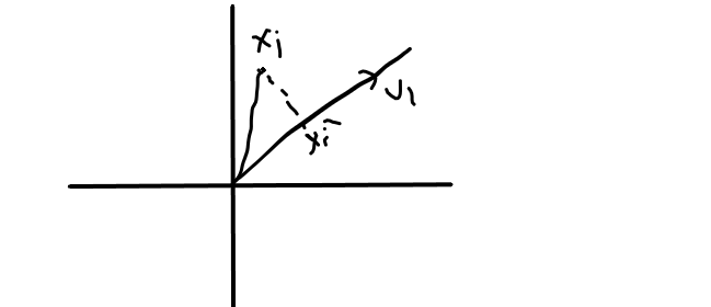
from image,

U1 is the direction, Xi is a point and Xi’ is the projection of Xi on U1,

Xi’ = proj_U1Xi ……   { proj_U1Xi = U1.Xi / ||U1|| }

Xi’ = U1.Xi / ||U1|| ……….    { ||U1|| = 1 }

Xi’ = U1.Xi

So, given any point Xi our projection is,

 >> Xi’ = U1^TXi  

 when we compute mean vector for Xi’ then the equation follow this:

>>  Xi’ ^ mean = U1^TXi

Our task is to find the U1 such that the var { proj_U1Xi } is maximum,

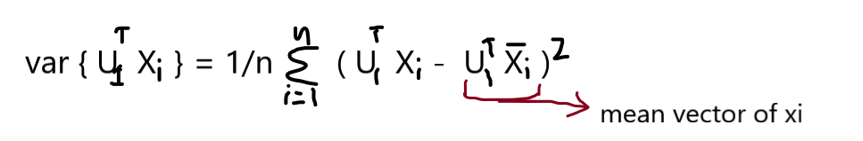
We know that the data matrix X is column standardized so our mean is 0 and variance is 1, So the data points of the mean vector are zeros,

x̄i = [0,0,0,……,0]

From the above consideration you know that we will use a unit vector to find the direction and then project the points onto the directed axis, but how do we find the unit vector direction where the variance is maximum. Many of us remember the term Eigen Values and Eigen Vectors this both concepts play important role in finding the direction of the axis.

Eigenvalues:-  It reveals that how much spread/variance in the data in that specific direction

Eigenvectors:-  It determines the direction of the new data points in the axis.

Every eigenvalue have corresponding eigenvectors,

IMAGE…

We have squared symmetric matrix of d X d and compute the eigen values then we will get d igen values ,

S_dxd = { λ1, λ2, λ3, λ4,……..λn }

corresponding vectors,

S_dxd = { v1, v2, v3, v4,……..v_n }

When we find the eigenvector then we also find our direction in which the variance is maximum.

So,

  U1 = V1 where U1 is the unit vector and V1 is the eigenvector with corresponding eigenvalues.

 The Eigenvector with the highest Eigenvalues is our principle component.

  Recall the steps

1. Column standardization of our dataset

2. Construct the covariance matrices from the standardized data

3. Finding the eigenvalues and eigenvectors

4. Find the eigenvector with the corresponding maximum eigenvalue

5. Choose those features which have high variance.

End Notes

we have learned the mathematics behind the principle component analysis, how the PCA works in black-box. How the higher school maths is used for dimensionality reduction.

For any queries please free to ask me.

Thank You.

LinkedIn:- Mayur Badole

Read my other articles also:- https://www.analyticsvidhya.com/blog/author/mayurbadole2407/

The media shown in this article are not owned by Analytics Vidhya and are used at the Author’s discretion.

Mayur Badole 27 Jul 2021