Practicing Your Deep Learning Skills- a Hands-On Project with Keras

This article was published as a part of the Data Science Blogathon

Introduction

If you want to excel in the field of Data Science, then always have to remember that the best way to learn Data Science is to apply Data Science – Link

As we all know that Keras has become a powerful and easy-to-use Python library that is used for building and evaluating Deep Learning models. It does not work alone but wraps the other efficient numerical computation libraries such as Theano, CNTK, and TensorFlow and allows us to define and train neural network models in a few lines of code. So, In this article, we will create a neural network model in Python using Keras. The questions on which we are going to focus specifically in this article are as follows:

• How to load a dataset for use with Keras?
• How to define, compile and train a Multilayer Perceptron model in Keras?
• How to evaluate a Keras model on a validation dataset?
• How to use the concept of model Checkpoints in Keras?
• How to save the models and how do reuse the saved model in our other problems?

                                                    Image Source: Link

Note: To follow this article properly you should have a basic understanding of artificial neural networks. If you are a beginner and you don’t have a better understanding of Artificial neural networks, firstly you can refer to the following article and then start with this for a better understanding:

Understanding and Implementing Artificial Neural Networks with Python and R

On the other hand, if you have a proper understanding of ANN, then you can refer to the following link to revise all the concepts of Artificial Neural Networks:

Test Your Skills on Artificial Neural Networks

So, without any further delay, let’s get started with our implementation part! 👇

Load the Necessary Libraries

The first step is to load the required Python libraries. We will import the following libraries:

• Numpy for optimizing the matrix multiplications,
• Matplotlib for data visualization purposes like plotting the images,
• The sequential model provides us an empty box in which we are adding several dense (i.e, fully connected) layers according to our required architecture,
• Dense to produce the fully connected layers in our neural network,
• MNIST to import the dataset from Keras directly, and
• to_categorical is to convert our labels in the form of one-hot encoded vectors.

import numpy 
import matplotlib.pyplot as plt
from tensorflow.keras.models import Sequential
from tensorflow.keras.layers import Dense
from tensorflow.keras.utils import to_categorical
from tensorflow.keras.datasets import mnist

Load Dataset in Numpy Format

In this article, we will be using the MNIST handwritten digits dataset, which is a simple computer vision dataset. It also includes labels for each image. Each image in this dataset is 28 pixels by 28 pixels.

Let’s have a look at some of the images from the MNIST dataset:

For our problem statement, we will split our dataset into two parts:

• Training Dataset: This contains 60,000 data points.
• Testing Dataset: This contains 10,000 data points.

(X_train, y_train), (X_test, y_test) = mnist.load_data()

Output:

X_train.shape
y_train.shape
X_test.shape
y_test.shape

Output:

(60000, 28, 28)
(60000, )
(10000, 28, 28)
(10000, )

Plot Four Images as a Grey Scale Image

Now, we will plot some of the images from our dataset using the matplotlib library, and specifically, we are using the subplot function of the matplotlib library.

# Plot 4 images as gray scale
plt.subplot(221)
plt.imshow(X_train[0], cmap=plt.get_cmap('gray'))
plt.subplot(222)
plt.imshow(X_train[1], cmap=plt.get_cmap('gray'))
plt.subplot(223)
plt.imshow(X_train[2], cmap=plt.get_cmap('gray'))
plt.subplot(224)
plt.imshow(X_train[3], cmap=plt.get_cmap('gray'))
# Show the plot
plt.show()

Output:

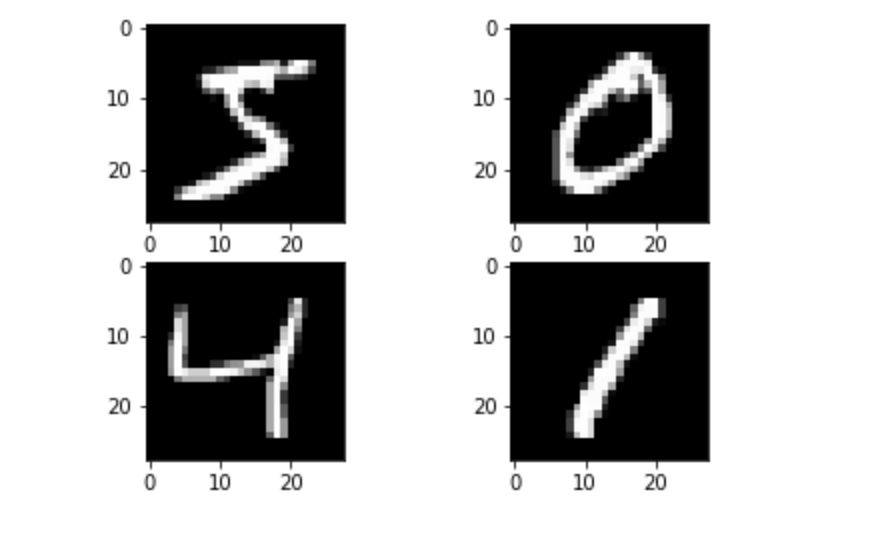
Image Source: Author

Formatting Data and Labels for Keras

Now, we will flatten our array of images into a vector of 28×28=784 numbers. As long as we’re consistent between images, it is irrespective of how we flatten the array. From this perspective, the images of the given dataset are just a bunch of points in a 784-dimensional vector space. But the data should always be of the format “(Number of data points, data point dimension)”. In this example, the training data will be of the dimension 60,000×784.

num_pixels = X_train.shape[1] * X_train.shape[2]
X_train = X_train.reshape(X_train.shape[0], num_pixels).astype('float32')
X_test = X_test.reshape(X_test.shape[0], num_pixels).astype('float32')
X_train = X_train / 255 
X_test = X_test / 255
y_train = to_categorical(y_train) 
y_test = to_categorical(y_test)
num_classes = y_test.shape[1]

Let’s again find the shape of our NumPy arrays with the following lines of codes:

X_train.shape
y_train.shape
X_test.shape
y_test.shape

Output:

(60000, 784)
(60000, 784)
(10000, 10)
(10000, 10)

Note: For our given problem statement, we will not only be using just one model instead we will be using different models having different architectures and finally we also compare the results of all the models which give you good clarity about the implementation part. The model architecture which we will be building in this article are as follows:

• Single Layer Neural Network
• Multi-Layer Neural Network
• Deep Neural Network

So, Let’s start with the first architecture (i.e, single-layer neural network): 🙂

Defining a single layer Neural Network Model

Here we will define a single-layer neural network. It will have an input layer of 784 neurons, i.e. the input dimension and output layer of 10 neurons, i.e. a number of classes. The activation function used will be softmax activation.

# create model
model = Sequential()  
model.add(Dense(num_classes, input_dim=num_pixels, activation='softmax'))

Compiling the Model

Once we defined our first model, our next step is to compile it. While compiling we have to give the loss function to be used, the optimizer, and any metric as an input. Here we will use

• Cross-entropy loss as a loss function,
• SGD as an optimizer, and
• Accuracy as a metric.

# Compile model
model.compile(loss='categorical_crossentropy', optimizer='sgd', metrics=['accuracy'])

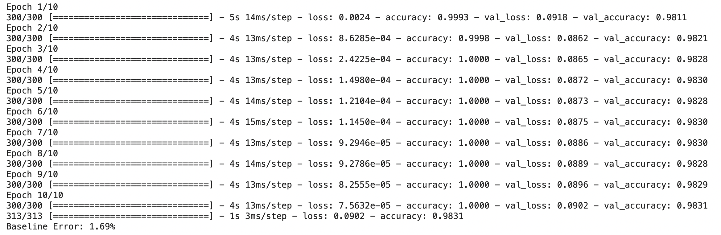
Training or Fitting the Model

After compilation, our model is ready to be trained. Now, we will provide training data to the neural network. Also, we have to specify the validation data, over which the model will only be validated along with the number of epochs and batch size as hyperparameters.

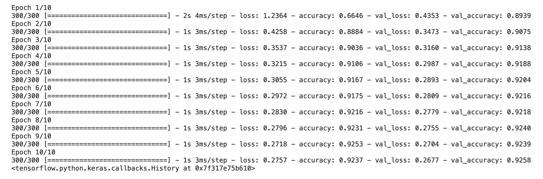
# Training model
model.fit(X_train, y_train, validation_data=(X_test, y_test), epochs=10, batch_size=200)

Output:

Evaluating the Model

Finally, we will evaluate the model on the testing dataset.

# Final evaluation of the model
scores = model.evaluate(X_test, y_test)
print("Baseline Error: %.2f%%" % (100-scores[1]*100))

Output:

Now, let’s start with the second architecture (i.e, multi-layer neural network): 🙂

Defining a Multi-Layer Neural Network Model

Now we will define a multi-layer neural network in which we will add 2 hidden layers having 500 and 100 neurons.

model = Sequential()
model.add(Dense(500, input_dim=num_pixels, activation='relu'))
model.add(Dense(100, activation='relu'))
model.add(Dense(num_classes, activation='softmax'))

Compiling the Model

Once we defined our second model, our next step is to compile it. While compiling we have to give the loss function to be used, the optimizer, and any metric as an input. Here we will use

• Cross-entropy loss as a loss function,
• Adam optimizer as an optimizer, and
• Accuracy as a metric.

# Compile model
model.compile(loss='categorical_crossentropy', optimizer='adam', metrics=['accuracy'])

Training or Fitting the Model

After compilation, our model is ready to be trained. Now, we will provide training data to the neural network. Also, we have to specify the validation data, over which the model will only be validated along with the number of epochs and batch size as hyperparameters.

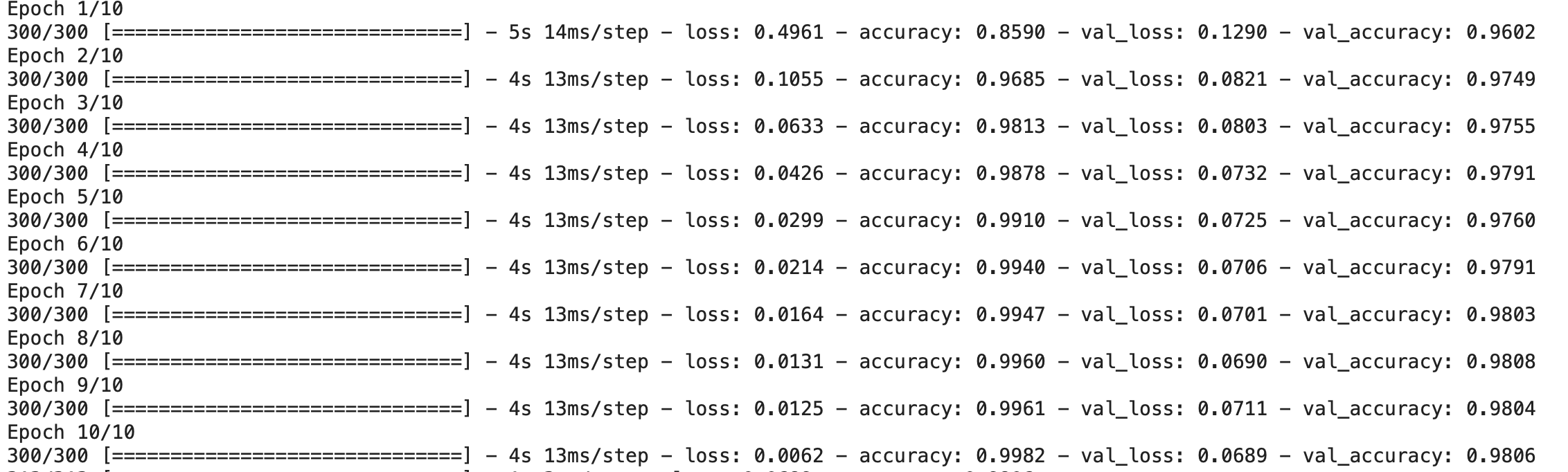
# Training model
model.fit(X_train, y_train, validation_data=(X_test, y_test), epochs=10, batch_size=200)

Output:

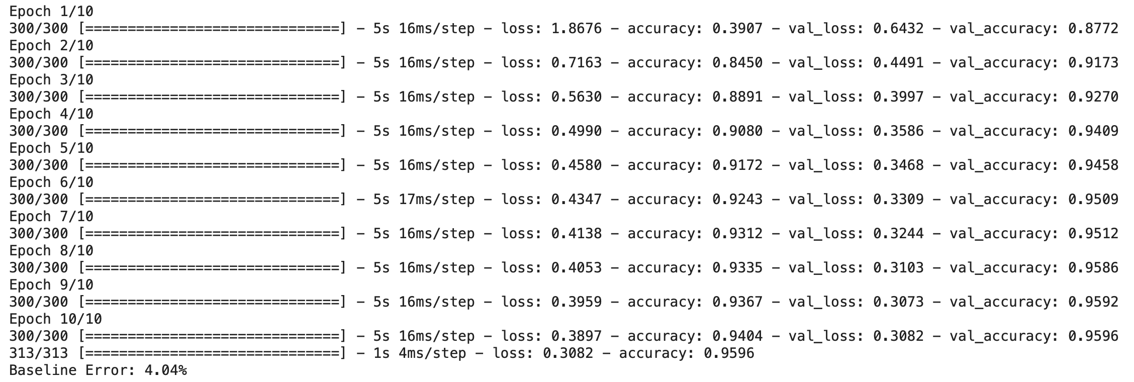
Evaluating the Model

Finally, we will evaluate the model on the testing dataset.

# Final evaluation of the model
scores = model.evaluate(X_test, y_test)
print("Baseline Error: %.2f%%" % (100-scores[1]*100))

Output:

Now, let’s start with the third architecture (i.e, deep neural network): 🙂

Defining a deep Neural Network Model

Now we will define a deep neural network in which we will add 3 hidden layers having 500, 100 and 50 neurons respectively.

model = Sequential()  
model.add(Dense(500, input_dim=num_pixels, activation='sigmoid'))
model.add(Dense(100, activation='sigmoid'))
model.add(Dense(50, activation = 'sigmoid'))
model.add(Dense(num_classes, activation='softmax'))

Compiling the Model

Once we defined our third model, our next step is to compile it. While compiling we have to give the loss function to be used, the optimizer, and any metric as an input. Here we will use

• Cross-entropy loss as a loss function,
• Adam optimizer as an optimizer, and
• Accuracy as a metric.

# Compile model
model.compile(loss='categorical_crossentropy', optimizer='adam', metrics=['accuracy'])

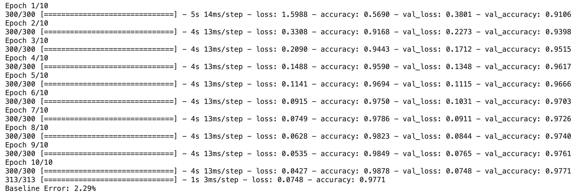
Training or Fitting the Model

After compilation, our model is ready to be trained. Now, we will provide training data to the neural network. Also, we have to specify the validation data, over which the model will only be validated along with the number of epochs and batch size as hyperparameters.

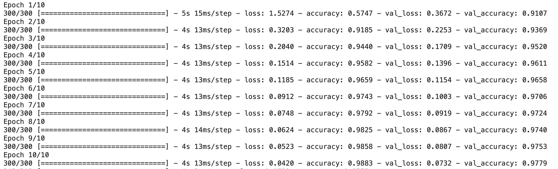
# Training model
model.fit(X_train, y_train, validation_data=(X_test, y_test), epochs=10, batch_size=200)

Output:

Evaluating the Model

Finally, we will evaluate the model on the testing dataset.

# Final evaluation of the model
scores = model.evaluate(X_test, y_test)
print("Baseline Error: %.2f%%" % (100-scores[1]*100))

Output:

 

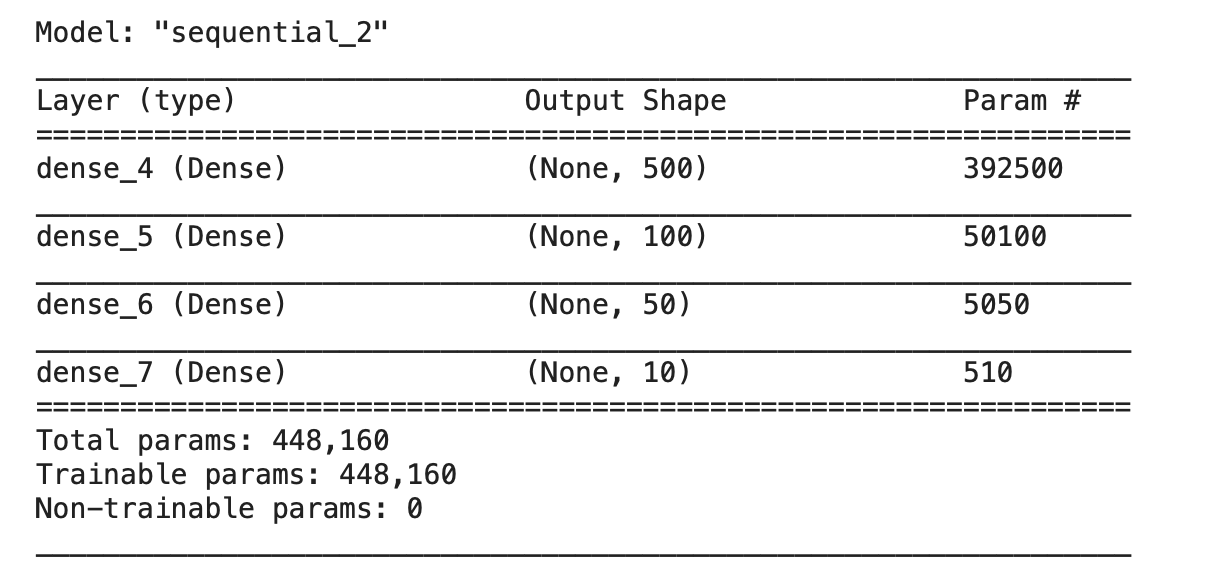
Analyzing Model Summary

The following function provides us with a detailed summary of the model. We can use it after we have defined our model.

model.summary()

Output:

 

Save the Model

In this section, we will save our model which we have build in the above section. To learn more about this, you can refer to the link.

import h5py
# Compile the model
model.compile(loss='categorical_crossentropy', optimizer='adam', metrics=['accuracy'])
# Training model
model.fit(X_train, y_train, validation_data=(X_test, y_test), epochs=10, batch_size=200)
model.save_weights('FC.h5')
# Final evaluation of the model
scores = model.evaluate(X_test, y_test)
print("Baseline Error: %.2f%%" % (100-scores[1]*100))

Output:

 

Loading the saved Model

Now, we will load the model which we have just saved and compare that with the random model. Here firstly we have created a random model and then load the previously saved model and compare the error of both.

model = Sequential()
model.add(Dense(500, input_dim=num_pixels, activation='sigmoid'))
model.add(Dense(100, activation='sigmoid'))
model.add(Dense(50, activation = 'sigmoid'))
model.add(Dense(num_classes, activation='softmax'))
# Compile model
model.compile(loss='categorical_crossentropy', optimizer='adam', metrics=['accuracy'])
# Final evaluation of the model
scores = model.evaluate(X_test, y_test)
print("Baseline Error: %.2f%%" % (100-scores[1]*100))

Output:

 

Now, load the saved model:

model.load_weights('FC.h5')
# Final evaluation of the model
scores = model.evaluate(X_test, y_test)
print("Baseline Error: %.2f%%" % (100-scores[1]*100))

Output:

 

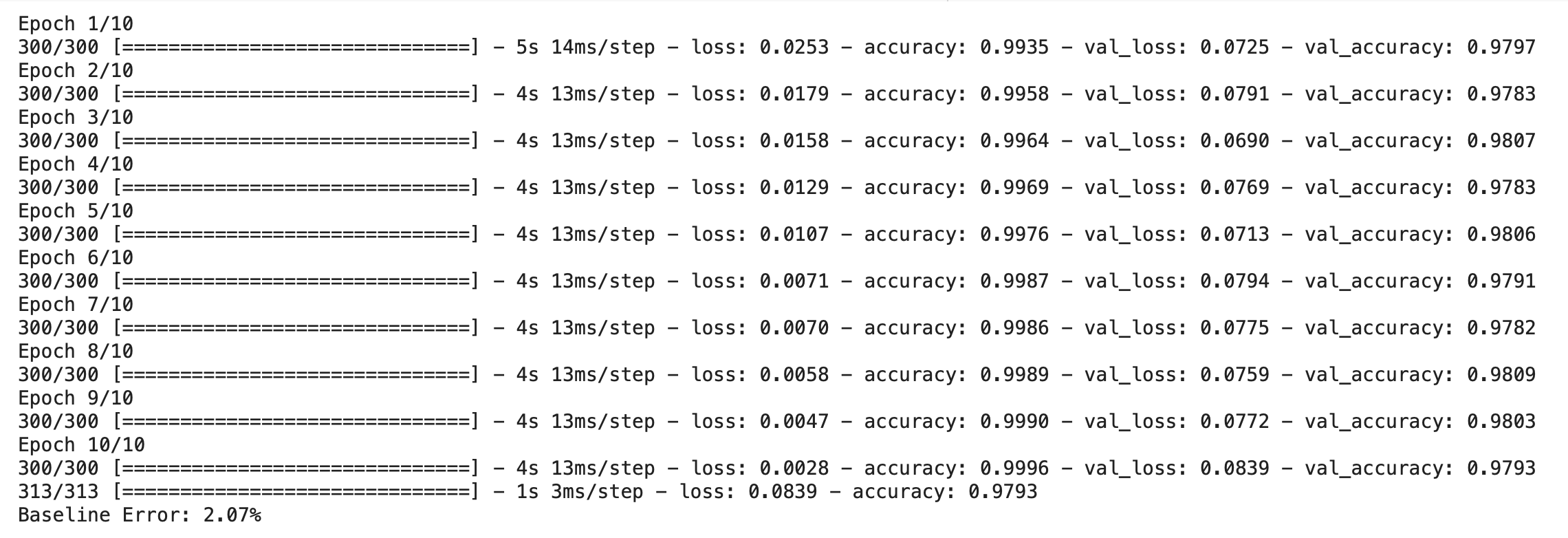
Creating checkpoints of Model

Here we make the model checkpoints (i.e, point after that there is no significant reduction in the validation error) and saved the weights of that point and used further wherever required.

from tensorflow.keras.callbacks import ModelCheckpoint
filepath='FC.h5'
checkpoint = ModelCheckpoint(filepath, monitor='val_accuracy', save_best_only=True, mode='max')
callbacks_list = [checkpoint]
model.fit(X_train, y_train, validation_data=(X_test, y_test), epochs=10, batch_size=200, callbacks=callbacks_list)

Output:

 

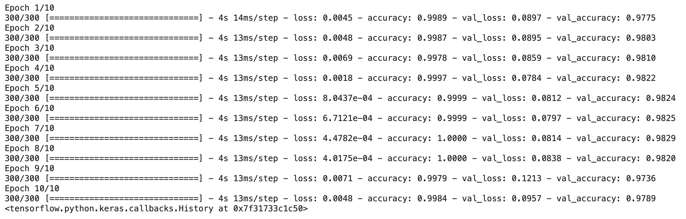
Defining Learning Rate Decay and Other Parameters of Optimizer

Now, we will use the SGD and Adam Optimizer for our model. To know more about the optimizers and their different types, you can refer to the following link:

Complete Guide to Optimizers in Deep Learning

from tensorflow.keras.optimizers import SGD, Adam
sgd = SGD(lr = 0.001, momentum = 0.0005, decay = 0.0005)   # 0.001  to 0.000001
adam = Adam(lr=0.001, beta_1=0.9, beta_2=0.999, epsilon=None, decay=0.0005)
model.compile(loss='categorical_crossentropy', optimizer=adam, metrics=['accuracy'])
# model.compile(loss='categorical_crossentropy', optimizer=sgd, metrics=['accuracy'])
model.fit(X_train, y_train, validation_data=(X_test, y_test), epochs=10, batch_size=200)
# Final evaluation of the model
scores = model.evaluate(X_test, y_test)
print("Baseline Error: %.2f%%" % (100-scores[1]*100))

Output:

Defining Regularizers for the Model

In this section, we will regularize our model. To learn about regularization and different types of methods by which we can regularize our neural networks, please refer to the given article:

Complete Guide to Regularization in Neural Networks

from tensorflow.keras import regularizers
from tensorflow.keras.layers import Dropout
model = Sequential() 
model.add(Dense(500, input_dim=num_pixels, activation='sigmoid', kernel_regularizer=regularizers.l2(1e-4)))
model.add(Dropout(0.3))
model.add(Dense(100, activation='sigmoid', kernel_regularizer=regularizers.l2(1e-4)))
model.add(Dropout(0.25))
model.add(Dense(50, activation = 'sigmoid', kernel_regularizer=regularizers.l2(1e-4)))
model.add(Dropout(0.3))
model.add(Dense(num_classes, activation='softmax', kernel_regularizer=regularizers.l2(1e-4)))
# Compile model
from tensorflow.keras.callbacks import ModelCheckpoint
model.compile(loss='categorical_crossentropy', optimizer='adam', metrics=['accuracy'])
# Training model
model.fit(X_train, y_train, validation_data=(X_test, y_test), epochs=10, batch_size=200)
# Final evaluation of the model
scores = model.evaluate(X_test, y_test)
print("Baseline Error: %.2f%%" % (100-scores[1]*100))

Output:

Defining Initialization for the Model

Here we will add dropout regularization and glorot weight initialization technique in the model. To learn about weight initialization and different types of methods by which we can initialize our neural networks, please refer to the given article:

How to Initialize Artificial Neural Networks?

from tensorflow.keras import initializers
from tensorflow.keras.layers import Dropout
model = Sequential()
model.add(Dense(500, input_dim=num_pixels, activation='sigmoid', kernel_initializer=initializers.GlorotNormal()))
model.add(Dense(100, activation='sigmoid', kernel_initializer=initializers.GlorotNormal()))
model.add(Dense(50, activation = 'sigmoid', kernel_initializer=initializers.GlorotNormal()))
model.add(Dense(num_classes, activation='softmax', kernel_initializer=initializers.GlorotNormal()))
# Compile model
from tensorflow.keras.callbacks import ModelCheckpoint
model.compile(loss='categorical_crossentropy', optimizer='adam', metrics=['accuracy'])
# Training model
model.fit(X_train, y_train, validation_data=(X_test, y_test), epochs=10, batch_size=200)
# Final evaluation of the model
scores = model.evaluate(X_test, y_test)
print("Baseline Error: %.2f%%" % (100-scores[1]*100))

Output:

This ends our implementation of the Deep Learning Project! 🥳

If you want to look at a similar kind of project, then you can refer to the following article:

Image Denoising Using AutoEncoders – Make your images clearer and crisper

Other Blog Posts by Me

You can also check my previous blog posts.

Previous Data Science Blog posts.

LinkedIn

Here is my Linkedin profile in case you want to connect with me. I’ll be happy to be connected with you.

Email

For any queries, you can mail me on Gmail.

End Notes

Thanks for reading!

I hope that you have enjoyed the article. If you like it, share it with your friends also. Something not mentioned or want to share your thoughts? Feel free to comment below And I’ll get back to you. 😉

The media shown in this article are not owned by Analytics Vidhya and are used at the Author’s discretion.

CHIRAG GOYAL 27 Jul 2021

I am currently pursuing my Bachelor of Technology (B.Tech) in Computer Science and Engineering from the Indian Institute of Technology Jodhpur(IITJ). I am very enthusiastic about Machine learning, Deep Learning, and Artificial Intelligence. Feel free to connect with me on Linkedin.