New to machine learning? Explore Logistic Regression with us, a beginner-friendly approach to predictive modeling. We’ll break down the basics, show you practical uses, and make it easy for you to apply in real-life situations. Let’s learn together!
Well, these were a few of my doubts when I was learning Logistic Regression . To find the math behind this, I plunged deeper into this topic only to find myself a better understanding of the Logistic Regression model. And in this article, I will try to answer all the doubts you are having right now on this topic. I will tell you the math behind this Logistic regression model.
Logistic regression is the appropriate regression analysis to conduct when the dependent variable is dichotomous (binary). Like all regression analyses, logistic regression is a predictive analysis. It is used to describe data and to explain the relationship between one dependent binary variable and one or more nominal, ordinal, interval or ratio-level independent variables.
I found this definition on google and now we’ll try to understand it. Logistic Regression is another statistical analysis method borrowed by Machine Learning. It is used when our dependent variable is dichotomous or binary. It just means a variable that has only 2 outputs, for example, A person will survive this accident or not, The student will pass this exam or not. The outcome can either be yes or no (2 outputs). This regression technique is similar to linear regression and can be used to predict the Probabilities for classification problems.
Types of Logistic Regression
Binary logistic regression
Binary logistic regression is used to predict the probability of a binary outcome, such as yes or no, true or false, or 0 or 1. For example, it could be used to predict whether a customer will churn or not, whether a patient has a disease or not, or whether a loan will be repaid or not.
Multinomial logistic regression
Multinomial logistic regression is used to predict the probability of one of three or more possible outcomes, such as the type of product a customer will buy, the rating a customer will give a product, or the political party a person will vote for.
Ordinal logistic regression
is used to predict the probability of an outcome that falls into a predetermined order, such as the level of customer satisfaction, the severity of a disease, or the stage of cancer.
Why do we use Logistic Regression rather than Linear Regression?
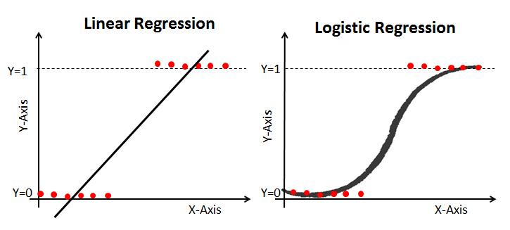
If you have this doubt, then you’re in the right place, my friend. After reading the definition of logistic regression we now know that it is only used when our dependent variable is binary and in linear regression this dependent variable is continuous.
The second problem is that if we add an outlier in our dataset, the best fit line in linear regression shifts to fit that point.
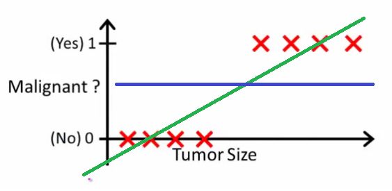
Now, if we use linear regression to find the best fit line which aims at minimizing the distance between the predicted value and actual value, the line will be like this:
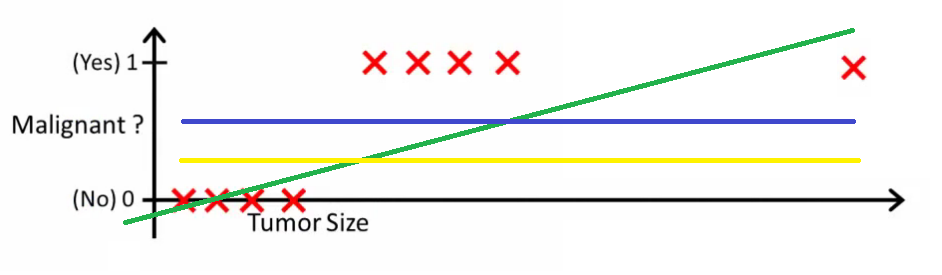
Here the threshold value is 0.5, which means if the value of h(x) is greater than 0.5 then we predict malignant tumor (1) and if it is less than 0.5 then we predict benign tumor (0). Everything seems okay here but now let’s change it a bit, we add some outliers in our dataset, now this best fit line will shift to that point. Hence the line will be somewhat like this:
Do you see any problem here? The blue line represents the old threshold and the yellow line represents the new threshold which is maybe 0.2 here. To keep our predictions right we had to lower our threshold value. Hence we can say that linear regression is prone to outliers. Now here if h(x) is greater than 0.2 then only this regression will give correct outputs.
Another problem with linear regression is that the predicted values may be out of range. We know that probability can be between 0 and 1, but if we use linear regression this probability may exceed 1 or go below 0.
To overcome these problems we use Logistic Regression, which converts this straight best fit line in linear regression to an S-curve using the sigmoid function, which will always give values between 0 and 1. How does this work and what’s the math behind this will be covered in a later section?
If you want to know the difference between logistic regression and linear regression then you refer to this article.
How does Logistic Regression work?
Logistic regression works in the following steps:
Prepare the data: The data should be in a format where each row represents a single observation and each column represents a different variable. The target variable (the variable you want to predict) should be binary (yes/no, true/false, 0/1).
Train the model: We teach the model by showing it the training data. This involves finding the values of the model parameters that minimize the error in the training data.
Evaluate the model: The model is evaluated on the held-out test data to assess its performance on unseen data.
Use the model to make predictions: After the model has been trained and assessed, it can be used to forecast outcomes on new data.
Logistic Function
You must be wondering how logistic regression squeezes the output of linear regression between 0 and 1. If you haven’t read my article on Linear Regression then please have a look at it for a better understanding.
Well, there’s a little bit of math included behind this and it is pretty interesting trust me.
Let’s start by mentioning the formula of logistic function:
How similar it is too linear regression? If you haven’t read my article on Linear Regression, then please have a look at it for a better understanding.
Best Fit Equation in Linear Regression
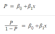
We all know the equation of the best fit line in linear regression is:
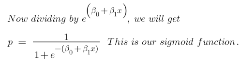
Let’s say instead of y we are taking probabilities (P). But there is an issue here, the value of (P) will exceed 1 or go below 0 and we know that range of Probability is (0-1). To overcome this issue we take “odds” of P:
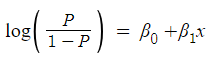
Do you think we are done here? No, we are not. We know that odds can always be positive which means the range will always be (0,+∞ ). Odds are nothing but the ratio of the probability of success and probability of failure. Now the question comes out of so many other options to transform this why did we only take ‘odds’? Because odds are probably the easiest way to do this, that’s it.
The problem here is that the range is restricted and we don’t want a restricted range because if we do so then our correlation will decrease. By restricting the range we are actually decreasing the number of data points and of course, if we decrease our data points, our correlation will decrease. It is difficult to model a variable that has a restricted range. To control this we take the log of oddswhich has a range from (-∞,+∞).
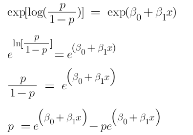
If you understood what I did here then you have done 80% of the maths. Now we just want a function of P because we want to predict probability right? not log of odds. To do so we will multiply by exponent on both sides and then solve for P.
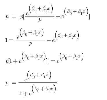
Now we have our logistic function, also called a sigmoid function. The graph of a sigmoid function is as shown below. It squeezes a straight line into an S-curve.
Key properties of the logistic regression equation
Sigmoid Function: The logistic regression model, when explained, uses a special “S” shaped curve to predict probabilities. It ensures that the predicted probabilities stay between 0 and 1, which makes sense for probabilities.
Straightforward Relationship: Even though the logistic regression model might seem complex, the relationship between our inputs (like age, height, etc.) and the outcome (like yes/no) is pretty simple to understand. It’s like drawing a straight line, but with a curve instead.
Coefficients: These are just numbers that tell us how much each input affects the outcome in the logistic regression model. For example, if age is a predictor, the coefficient tells us how much the outcome changes for every one year increase in age.
Best Guess: We figure out the best coefficients for the logistic regression model by looking at the data we have and tweaking them until our predictions match the real outcomes as closely as possible.
Basic Assumptions: In logistic regression explained, we assume that our observations are independent, meaning one doesn’t affect the other. We also assume that there’s not too much overlap between our predictors (like age and height), and the relationship between our predictors and the outcome is kind of like a straight line.
Probabilities, Not Certainties: Instead of saying “yes” or “no” directly, logistic regression gives us probabilities, like saying there’s a 70% chance it’s a “yes” in the logistic regression model. We can then decide on a cutoff point to make our final decision.
Checking Our Work: In logistic regression explained, we have some tools to make sure our predictions are good, like accuracy, precision, recall, and a curve called the ROC curve. These help us see how well our logistic regression model is doing its job.
Cost Function in Logistic Regression
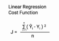
In linear regression, we use the Mean squared error which was the difference between y_predicted and y_actual and this is derived from the maximum likelihood estimator. The graph of the cost function in linear regression is like this:
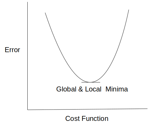
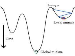
In logistic regression Yi is a non-linear function (Ŷ=1/1+ e-z). If we use this in the above MSE equation then it will give a non-convex graph with many local minima as shown
The problem here is that this cost function will give results with local minima, which is a big problem because then we’ll miss out on our global minima and our error will increase.
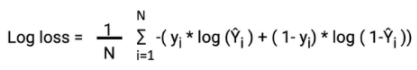
In order to solve this problem, we derive a different cost function for logistic regression called log loss which is also derived from the maximum likelihood estimation method.
In the next section, we’ll talk a little bit about the maximum likelihood estimator and what it is used for. We’ll also try to see the math behind this log loss function.
What is the use of Maximum Likelihood Estimator?
The primary objective of Maximum Likelihood Estimation (MLE) in machine learning, particularly in the context of logistic regression, is to identify parameter values that maximize the likelihood function. This function represents the joint probability density function (pdf) of our sample observations. In essence, it involves multiplying the conditional probabilities for observing each example given the distribution parameters. In the realm of logistic regression in machine learning, this process aims to discover parameter values such that, when plugged into the model for P(x), it produces a value close to one for individuals with a malignant tumor and close to zero for those with a benign tumor.
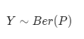
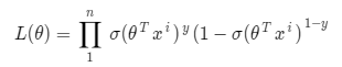
Let’s start by defining our likelihood function. We now know that the labels are binary which means they can be either yes/no or pass/fail etc. We can also say we have two outcomes success and failure. This means we can interpret each label as Bernoulli random variable.
Random Experiment
A random experiment whose outcomes are of two types, success S and failure F, occurring with probabilities p and q respectively is called a Bernoulli trial. If for this experiment a random variable X is defined such that it takes value 1 when S occurs and 0 if F occurs, then X follows a Bernoulli Distribution.
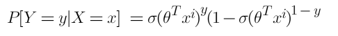
Where P is our sigmoid function
where σ(θ^T*x^i) is the sigmoid function. Now for n observations,
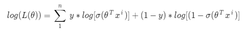
We need a value for theta which will maximize this likelihood function. To make our calculations easier we multiply the log on both sides. The function we get is also called the log-likelihood function or sum of the log conditional probability
In machine learning, it is conventional to minimize a loss(error) function via gradient descent, rather than maximize an objective function via gradient ascent. If we maximize this above function then we’ll have to deal with gradient ascent to avoid this we take negative of this log so that we use gradient descent. We’ll talk more about gradient descent in a later section and then you’ll have more clarity. Also, remember,
max[log(x)] = min[-log(x)]
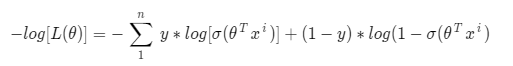
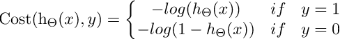
The negative of this function is our cost function and what do we want with our cost function? That it should have a minimum value. It is common practice to minimize a cost function for optimization problems; therefore, we can invert the function so that we minimize the negative log-likelihood (NLL). So in logistic regression, our cost function is:
Here y represents the actual class and log(σ(θ^T*x^i) ) is the probability of that class.
p(y) is the probability of 1.
1-p(y) is the probability of 0.
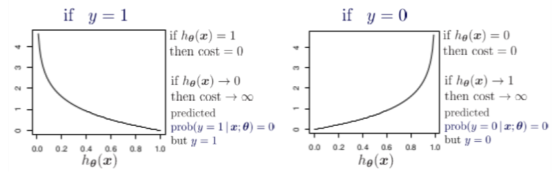
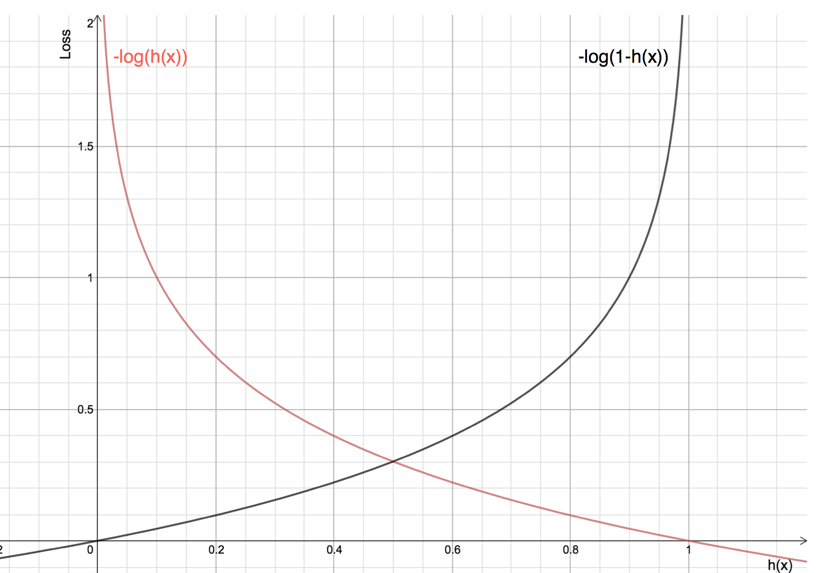
Let’s see what will be the graph of cost function when y=1 and y=0
If we combine both the graphs, we will get a convex graph with only 1 local minimum and now it’ll be easy to use gradient descent here.
The red line here represents the 1 class (y=1), the right term of cost function will vanish. Now if the predicted probability is close to 1 then our loss will be less and when probability approaches 0, our loss function reaches infinity.
The black line represents 0 class (y=0), the left term will vanish in our cost function and if the predicted probability is close to 0 then our loss function will be less but if our probability approaches 1 then our loss function reaches infinity.
This cost function is also called log loss. It also ensures that as the probability of the correct answer is maximized, the probability of the incorrect answer is minimized. Lower the value of this cost function higher will be the accuracy.
Gradient Descent Optimization
In this section, we will try to understand how we can utilize Gradient Descent to compute the minimum cost.
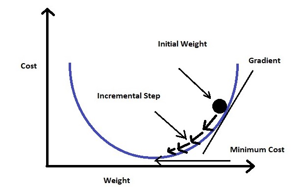
Gradient descent changes the value of our weights in such a way that it always converges to minimum point or we can also say that, it aims at finding the optimal weights which minimize the loss function of our model. It is an iterative method that finds the minimum of a function by figuring out the slope at a random point and then moving in the opposite direction.
The intuition is that if you are hiking in a canyon and trying to descend most quickly down to the river at the bottom, you might look around yourself 360 degrees, find the direction where the ground is sloping the steepest, and walk downhill in that direction.
At first gradient descent takes a random value of our parameters from our function. Now we need an algorithm that will tell us whether at the next iteration we should move left or right to reach the minimum point. The gradient descent algorithm finds the slope of the loss function at that particular point and then in the next iteration, it moves in the opposite direction to reach the minima. Since we have a convex graph now we don’t need to worry about local minima. A convex curve will always have only 1 minima.
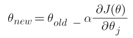
We can summarize the gradient descent algorithm as:
Here alpha is known as the learning rate. It determines the step size at each iteration while moving towards the minimum point. Usually, a lower value of “alpha” is preferred, because if the learning rate is a big number then we may miss the minimum point and keep on oscillating in the convex curve
Now the question is what is this derivative of cost function? How do we do this? Don’t worry, In the next section we’ll see how we can derive this cost function w.r.t our parameters.
Derivation of Cost Function:
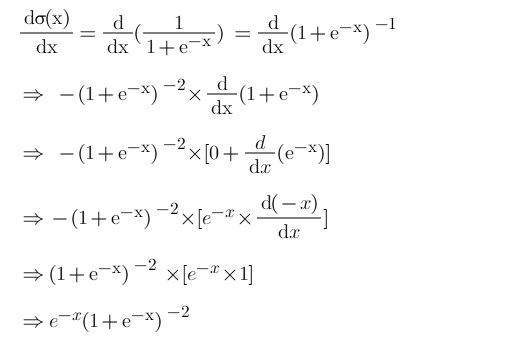
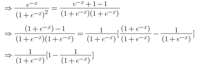
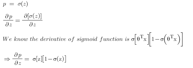
Before we derive our cost function we’ll first find a derivative for our sigmoid function because it will be used in derivating the cost function.
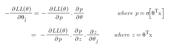
Now, we will derive the cost function with the help of the chain rule as it allows us to calculate complex partial derivatives by breaking them down.
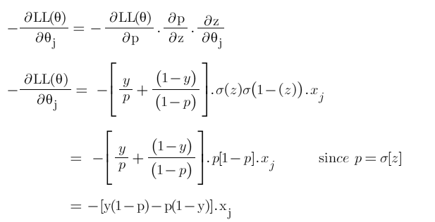
Step-1: Use chain rule and break the partial derivative of log-likelihood.
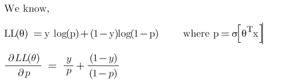
Step-2: Find derivative of log-likelihood w.r.t p
Step-3: Find derivative of ‘p’ w.r.t ‘z’
Step-4: Find derivate of z w.r.t θ
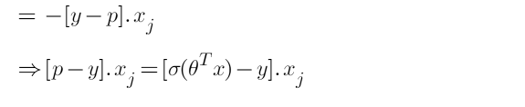
Step-5: Put all the derivatives in equation 1
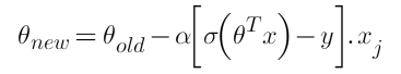
Hence the derivative of our cost function is:
Now since we have our derivative of the cost function, we can write our gradient descent algorithm as:
If the slope is negative (downward slope) then our gradient descent will add some value to our new value of the parameter directing it towards the minimum point of the convex curve. Whereas if the slope is positive (upward slope) the gradient descent will minus some value to direct it towards the minimum point.
Conclusion
To summarize, in this article, we explored the limitations of linear regression in addressing classification problems. Naturally, we delved into the application of Maximum Likelihood Estimation (MLE) in logistic regression and derived the associated cost function. In the upcoming article, we will comprehensively discuss the interpretations of logistic regression in machine learning and explore methods to assess the accuracy of our logistic model.
In the next article, I will explain all the interpretations of logistic regression. And how we can check the accuracy of our logistic model.
Let me know if you have any queries in the comments below.
Frequently Asked Questions
Q1. Is logistics regression vs linear regression?
Logistic regression, also known as logistics regression, is used for categorical outcomes, while linear regression is used for continuous outcomes.
Q2. What is Better than Logistics Regression?
There are a number of machine learning algorithms that can outperform logistic regression on certain tasks. For example, random forests and gradient-boosting machines can often achieve higher accuracy on classification tasks. However, logistic regression is still a very popular algorithm due to its simplicity, interpretability, and efficiency.
Q3. What is a key characteristic of logistic regression Explained?
A key characteristic of logistic regression, also referred to as logistics regression, is its suitability for binary classification problems where the outcome variable has two categories.
Q4. What is the main assumption of logistic regression?
The main assumption of logistic regression, often termed as logistics regression, is that the relationship between independent variables and the log odds of the dependent variable is linear.
The media shown in this article are not owned by Analytics Vidhya and are used at the Author’s discretion.
I am an undergraduate student currently in my last year majoring in Statistics (Bachelors of Statistics) and have a strong interest in the field of data science, machine learning, and artificial intelligence. I enjoy diving into data to discover trends and other valuable insights about the data. I am constantly learning and motivated to try new things.
Great presentation, very precise and concise with relevant examples. Kudos!
Anurag Tomar
30 Jul, 2022
The best article on logisitic regression, explained everything from the very basic
Ken
22 Sep, 2022
This is a really good write up and I enjoyed using this to review. I noticed a typo in step 5 of deriving the log-likelihood in the second line. It says sigmoid(1-(z)) but it should say (1-sigmoid(z)) which is how you get 1-p on the next line
A verification link has been sent to your email id
If you have not recieved the link please goto
Sign Up page again
Loading...
Please enter the OTP that is sent to your registered email id
Loading...
Please enter the OTP that is sent to your email id
Loading...
Please enter your registered email id
This email id is not registered with us. Please enter your registered email id.
Don't have an account yet?Register here
Loading...
Please enter the OTP that is sent your registered email id
Loading...
Please create the new password here
We use cookies on Analytics Vidhya websites to deliver our services, analyze web traffic, and improve your experience on the site. By using Analytics Vidhya, you agree to our Privacy Policy and Terms of Use.Accept
Privacy & Cookies Policy
Privacy Overview
This website uses cookies to improve your experience while you navigate through the website. Out of these, the cookies that are categorized as necessary are stored on your browser as they are essential for the working of basic functionalities of the website. We also use third-party cookies that help us analyze and understand how you use this website. These cookies will be stored in your browser only with your consent. You also have the option to opt-out of these cookies. But opting out of some of these cookies may affect your browsing experience.
Necessary cookies are absolutely essential for the website to function properly. This category only includes cookies that ensures basic functionalities and security features of the website. These cookies do not store any personal information.
Any cookies that may not be particularly necessary for the website to function and is used specifically to collect user personal data via analytics, ads, other embedded contents are termed as non-necessary cookies. It is mandatory to procure user consent prior to running these cookies on your website.


.jpg)


Great presentation, very precise and concise with relevant examples. Kudos!
The best article on logisitic regression, explained everything from the very basic
This is a really good write up and I enjoyed using this to review. I noticed a typo in step 5 of deriving the log-likelihood in the second line. It says sigmoid(1-(z)) but it should say (1-sigmoid(z)) which is how you get 1-p on the next line
Very Detailed and easy to understand.