Hierarchical Clustering Algorithm Python!
This article was published as a part of the Data Science Blogathon
Introduction
In this article, we’ll look at a different approach to K Means clustering called Hierarchical Clustering. In comparison to K Means or K Mode, hierarchical Clustering has a different underlying algorithm for how the clustering mechanism works. Hierarchical clustering uses agglomerative or divisive techniques, whereas K Means uses a combination of centroid and euclidean distance to form clusters. Dendrograms can be used to visualize clusters in hierarchical clustering, which can help with a better interpretation of results through meaningful taxonomies. We don’t have to specify the number of clusters when making a dendrogram.
Here we use Python to explain the Hierarchical Clustering Model. We have 200 mall customers’ data in our dataset. Each customer’s customerID, genre, age, annual income, and spending score are all included in the data frame. The amount computed for each of their clients’ spending scores is based on several criteria, such as their income, the number of times per week they visit the mall, and the amount of money they spent in a year. This score ranges from 1 to 100. Because we don’t know the answers, a business problem becomes a clustering problem. The data’s final categories are unknown to us. As a result, our goal is to discover some previously unknown customer clusters.
But first, we look into some important terms in hierarchical clustering.
Important Terms in Hierarchical Clustering
Linkage Methods
Single Linkage — The distances between the most similar members are calculated for each pair of clusters, and the clusters are then merged based on the shortest distance.
Average Linkage — The distance between all members of one cluster and all members of another cluster is calculated. After that, the average of these distances is used to determine which clusters will merge.
Median Linkage — We use the median distance instead of the average distance in a similar way to the average linkage.
Centroid Linkage — The centroid of each cluster is calculated by averaging all points assigned to the cluster, and the distance between clusters is then calculated using this centroid.
Distance Calculation
Multiple approaches to calculating distance between two or more clusters exist, with Euclidean Distance being the most popular. Other distance metrics, such as Minkowski, City Block, Hamming, Jaccard, and Chebyshev, can be used with hierarchical clustering as well. Different distance metrics have an impact on hierarchical clustering, as shown in Figure 2.
Dendrogram
The relationship between objects in a feature space is represented by a dendrogram. In a feature space, it’s used to show the distance between each pair of sequentially merged objects. Dendrograms are frequently used to examine hierarchical clusters before deciding on the appropriate number of clusters for the dataset. The dendrogram distance is the distance between two clusters when they combine. The dendrogram distance determines whether two or more clusters are disjoint or can be joined together to form a single cluster.
Example
Now we look into examples using Python to demonstrate the Hierarchical Clustering Model. We have 200 mall customers’ data in our dataset. Each customer’s customerID, genre, age, annual income, and spending score are all included in the data frame. The amount computed for each of their clients’ spending scores is based on several criteria, such as their income, the number of times per week they visit the mall, and the money they spent for a year. This score ranges from 1 to 100. Because we don’t know the answers, a business problem becomes a clustering problem.
This new step in hierarchical clustering also entails determining the optimal number of clusters. We’re not going to use the elbow method this time. We’ll make use of the dendrogram.
#3 Using the dendrogram to find the optimal numbers of clusters.
# First thing we're going to do is to import scipy library. scipy is an open source
# Python library that contains tools to do hierarchical clustering and building dendrograms.
# Only import the needed tool.
import scipy.cluster.hierarchy as sch
#Lets create a dendrogram variable
# linkage is actually the algorithm itself of hierarchical clustering and then in
#linkage we have to specify on which data we apply and engage. This is X dataset
dendrogram = sch.dendrogram(sch.linkage(X, method  = "ward"))
plt.title('Dendrogram')
plt.xlabel('Customers')
plt.ylabel('Euclidean distances')
plt.show()
The Ward method is a method that attempts to reduce variance within each cluster. It’s almost the same as when we used K-means to minimize the wcss to plot our elbow method chart; the only difference is that instead of wcss, we’re minimizing the within-cluster variants. Within each cluster, this is the variance. The dendrogram is shown below.
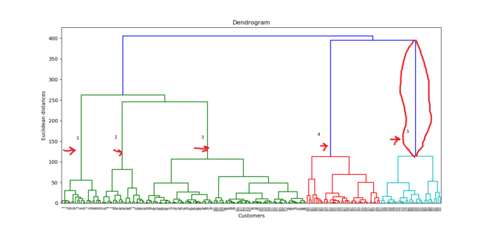
Customers are represented on the x-axis, and the Euclidean distance between clusters is represented on the y-axis. How do we figure out the best number of clusters based on this diagram? We want to find the longest vertical distance we can without crossing any horizontal lines, which is the red-framed line in the diagram above. Let’s count the lines on the diagram and figure out how many clusters are best. For this dataset, the cluster number will be 5.
#4 Fitting hierarchical clustering to the Mall_Customes dataset
# There are two algorithms for hierarchical clustering: Agglomerative Hierarchical Clustering and
# Divisive Hierarchical Clustering. We choose Euclidean distance and ward method for our
# algorithm class
from sklearn.cluster import AgglomerativeClustering
hc = AgglomerativeClustering(n_clusters = 5, affinity = 'euclidean', linkage ='ward')
# Lets try to fit the hierarchical clustering algorithm  to dataset X while creating the
# clusters vector that tells for each customer which cluster the customer belongs to.
y_hc=hc.fit_predict(X)
#5 Visualizing the clusters. This code is similar to k-means visualization code.
#We only replace the y_kmeans vector name to y_hc for the hierarchical clustering
plt.scatter(X[y_hc==0, 0], X[y_hc==0, 1], s=100, c='red', label ='Cluster 1')
plt.scatter(X[y_hc==1, 0], X[y_hc==1, 1], s=100, c='blue', label ='Cluster 2')
plt.scatter(X[y_hc==2, 0], X[y_hc==2, 1], s=100, c='green', label ='Cluster 3')
plt.scatter(X[y_hc==3, 0], X[y_hc==3, 1], s=100, c='cyan', label ='Cluster 4')
plt.scatter(X[y_hc==4, 0], X[y_hc==4, 1], s=100, c='magenta', label ='Cluster 5')
plt.title('Clusters of Customers (Hierarchical Clustering Model)')
plt.xlabel('Annual Income(k$)')
plt.ylabel('Spending Score(1-100')
plt.show()
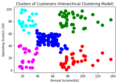
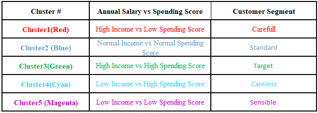
These clusters can be thought of as the mall’s customer segment.
That’s all there is to a standard Hierarchical Clustering Model. The dataset as well as all of the codes are available in the Github section.
Conclusion
In any clustering exercise, determining the number of clusters is a time-consuming process. Because the commercial side of the business is more concerned with extracting meaning from these groups, it’s crucial to visualize the clusters in two dimensions and see if they’re distinct. PCA or Factor Analysis can be used to achieve this goal. This is a common method for presenting final results to various stakeholders, making it easier for everyone to consume the output.
EndNote
Thank you for reading!
I hope you enjoyed the article and increased your knowledge.
Please feel free to contact me on Email
Something not mentioned or want to share your thoughts? Feel free to comment below And I’ll get back to you.
About the Author
Hardikkumar M. Dhaduk
Data Analyst | Digital Data Analysis Specialist | Data Science Learner
Connect with me on Linkedin
Connect with me on Github


