Performance Comparison of Regularized and Unregularized Regression Models
This article was published as a part of the Data Science Blogathon
Introduction
Regularization came out to be an essential technique for reducing the effect of overfitting, especially for regression problems. An overfitting model has a large variation in Train set Root Mean Square Error (RMSE) and test Root Mean Square Error (RMSE). Regularized Regression Model tends to show the least difference between the Train and Test Set RMSE than the Classical Regression Model.
In this article, we will focus on performance evaluation and comparison of Unregularized Classical Multilinear Regression Models with Regularized Multilinear Regression Models on a dataset. We will compare the RMSE for Train and Test set and will try to determine which Regression Model performs the best for the given dataset. We are going to use four Regression Models, Linear Regression Model, Lasso Regression Model, Ridge Regression Model, and ElasticNet Regression Model.

Table of Contents
- Regularization in Regression Model
- Unregularized Regression Model Performace
- Regularized Regression Model Performace
- Conclusions
Regularization in Regression Model
Regularization in Linear regression is a technique that prevents overfitting in the model by penalizing the coefficients involved in the linear regression equation. Coefficients in an overfitted model are inflated or weigh highly. Thus adding penalties on these parameters prevent them from inflating. Overfitted Models perform well on the training data while fail to perform on the test or new data passed. Thus, the built model has no use. We add coefficients to the cost function which is the Mean Squared Error (Sum of Squared Residuals Divided by Degrees of Freedom) of the regression model, which as a result increases the cost. The optimizer would try to minimize the coefficient to decrease the cost function. In regularization, penalizes all the parameters except the intercept.
Two Regularization techniques can be used to present overfitting. The L1 Regularization or LASSO adds the absolute value of coefficients as penalties to the cost function. The L2 Regularization or Ridge adds the summation of squared values of coefficients as penalities to the cost function. The alpha value represents how much we want to penalize the coefficients.
The unregularized Regression Model is our Classical Linear (or Multilinear) Regression Model. While Regularized Regression Models are based on these Regularization techniques. The Ridge Regression Model is based on the L2 Regularization Technique. While Lasso Regression Model is based on the L1 Regularization technique. The ElasticNet Regression Model is based on both L1 and L2 Regularization techniques. Let’s compare the performances of the Unregularized Regression Models with Regularized Regression Models.
Unregularized Regression Model Performace
Here, we will build a Classic Multilinear Regression Model for the specified dataset. We will calculate the Train and Test RMSE and later will compare with Regularized Regression Models.
Importing the libraries and Dataset
The dataset has been taken from Kaggle
Specifying the x and y variables
x = df.drop('Weight', axis = 1)
y = df['Weight']
y = y.values.reshape(-1,1)
For this dataset, our task is to predict the Weight of the Fishes based on several features. Thus, ‘Weight’ is our target feature. For the x variable, we are taking every feature except the target variable ‘Weight’ and for the y variable, we are taking just the target ‘Weight’.
Creating Dummies for Categorical Features
x = pd.get_dummies(x, drop_first = True)
Since our dataset contains a categorical feature, we will use the .get_dummies() method of pandas to create dummies for the unique classes of the categorical feature. Set the drop_first parameter value to True to save ourselves from the dummy variable trap.
Creating Train and Test Split
x_train, x_test, y_train, y_test = train_test_split(x, y, test_size = 0.3, random_state = 66)
Creating train and test sets for x and y variables using train_test_split module
Building a Linear Regression Model
linreg = LinearRegression()
Here we created an object linreg for the module LinearRegression from the sklearn library.
Fitting Model with x and y train sets
linreg.fit(x_train, y_train)
Calculating Train and Test Set RMSE
print("Train RMSE:", np.round(np.sqrt(metrics.mean_squared_error(y_train, linreg.predict(x_train))), 5))
print("Test RMSE:", np.round(np.sqrt(metrics.mean_squared_error(y_test, linreg.predict(x_test))), 5))
We are using the mean_squared_error method of the metrics module from the sklearn library. It takes the actual y and the predicted y arguments. For the Train RMSE, we used y_train as the actual y value and linreg.predict(x_train) method for the predicted y
value. For the Test RMSE, we used y_test as the actual y value and linreg.predict(x_test) method for the predicted y value. The .predict()
method of LinearRegression predicts the y value for the given x values (here
x_train and x_test).
Putting it all Together
import numpy as np
import pandas as pd
from sklearn.model_selection import train_test_split
from sklearn.linear_model import LinearRegression
from sklearn import metrics
import warnings
warnings.filterwarnings('ignore')
df = pd.read_csv('Fish.csv')
x = df.drop('Weight', axis = 1)
y = df['Weight']
y = y.values.reshape(-1,1)
x = pd.get_dummies(x, drop_first = True)
x_train, x_test, y_train, y_test = train_test_split(x, y, test_size = 0.3, random_state = 66)
linreg = LinearRegression()
linreg.fit(x_train, y_train)
print("Train RMSE:", np.round(np.sqrt(metrics.mean_squared_error(y_train, linreg.predict(x_train))), 5))
print("Test RMSE:", np.round(np.sqrt(metrics.mean_squared_error(y_test, linreg.predict(x_test))), 5))
On executing this, we get:
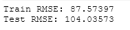
For the Classical Regression Model, Train Root Mean Square Error came out to be 87.57 while Test Root Mean Square Error came out to be 104.03. As discussed earlier, a perfect model often shows almost equal Train and Test Errors. Now, We will compare the difference between these Train and Test Error-values with Regularized Regression Models to provide our judgment if this Classical Regression Model is perfect or not.
Regularized Regression Model Performace
For the Regularized Regression Models, will look at LASSO Regression, Ridge Regression, and ElasticNet Regression and compare their performances (by checking the difference in Train-Test error values) with the performance of the Unregularized Classical Regression Model (Train-Test error values) evaluated above.
1. LASSO Regression
LASSO (or Least Least Absolute Shrinkage and Selection Operator) or L1 is a regularization technique in which the summation of absolute coefficient values is added to the cost function (or MSE) as a penalty. Lasso Regression is based on this L1 Regularization technique. Learn more about the Lasso Regression and L1 Regularization technique on Analytics Vidhya and here.
Now, let’s
build a Lasso Regression Model and evaluate the RMSE for Train and Test
Set.
Importing the libraries
import numpy as np
import pandas as pd
from sklearn.model_selection import train_test_split
from sklearn.linear_model import Lasso
from sklearn import metrics
import warnings
warnings.filterwarnings('ignore')
Importing the Dataset
df = pd.read_csv('Fish.csv')
The dataset has been taken from Kaggle
Specifying the x and y variables
x = df.drop('Weight', axis = 1)
y = df['Weight']
y = y.values.reshape(-1,1)
For this dataset, our task is to predict the Weight of the Fishes based on several features. Thus, ‘Weight‘ is our target feature. For the x
variable, we are taking every feature except the target variable ‘Weight’ and for y variable, we are taking just the target ‘Weight‘.
Creating Dummies for Categorical Variables
x = pd.get_dummies(x, drop_first = True)
Since our dataset contains a categorical feature, we will use the .get_dummies() method of pandas to create dummies for the unique classes of the categorical feature. Set the drop_first parameter value to True, to save ourselves from the dummy variable trap.
Creating Train and Test Sets
x_train, x_test, y_train, y_test = train_test_split(x, y, test_size = 0.3, random_state = 66)
Creating train and test sets for x and y variables using train_test_split module
Building a Lasso Regression Model
lasso = Lasso()
Here we created an object lasso for the module Lasso from the sklearn library.
Fitting Model with x and y train sets
lasso.fit(x_train, y_train)
Calculating Lasso Train and Test Set RMSE
print("Lasso Train RMSE:", np.round(np.sqrt(metrics.mean_squared_error(y_train, lasso.predict(x_train))), 5))
print("Lasso Test RMSE:", np.round(np.sqrt(metrics.mean_squared_error(y_test, lasso.predict(x_test))), 5))
We are using the mean_squared_error method of the metrics module from the sklearn library. It takes the actual y and the predicted y arguments. For the Train RMSE, we used y_train as the actual y value and lasso.predict(x_train) method for the predicted y value. For the Test RMSE, we used y_test as the actual y value and lasso.predict(x_test) method for the predicted y value. The .predict()
method of Lasso predicts the y value for the given x values (here
x_train and x_test).
Putting it all together
import numpy as np
import pandas as pd
from sklearn.model_selection import train_test_split
from sklearn.linear_model import Lasso
from sklearn import metrics
import warnings
warnings.filterwarnings('ignore')
df = pd.read_csv('Fish.csv')
x = df.drop('Weight', axis = 1)
y = df['Weight']
y = y.values.reshape(-1,1)
x = pd.get_dummies(x, drop_first = True)
x_train, x_test, y_train, y_test = train_test_split(x, y, test_size = 0.3, random_state = 66)
lasso = Lasso()
lasso.fit(x_train, y_train)
print("Lasso Train RMSE:", np.round(np.sqrt(metrics.mean_squared_error(y_train, lasso.predict(x_train))), 5))
print("Lasso Test RMSE:", np.round(np.sqrt(metrics.mean_squared_error(y_test, lasso.predict(x_test))), 5))
On executing this, we get:
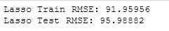
For the Lasso Regression Model, Train Root Mean Square Error came out to be 91.95. while Test Root Mean Square Error came out to be 95.98. As
discussed earlier, a perfect model often shows almost equal Train and
Test Errors. We will compare this difference of these Error terms with the Classical Regression Model and the rest of Regularized Regression Models.

2. Ridge Regression
Ridge or L2 is a Regularization Technique in which the summation of squared values of the coefficients of the regression equation is added as penalty into cost function (or MSE). Ridge Regression is based on the L2 Regularization technique. Learn more about the L2 Regularization technique and Ridge Regression on Analytics Vidhya and here.
Now, let’s build a Ridge Regression Model and evaluate the RMSE for Train and Test Set.
Importing the libraries
import numpy as np
import pandas as pd
from sklearn.model_selection import train_test_split
from sklearn.linear_model import Ridge
from sklearn import metrics
import warnings
warnings.filterwarnings('ignore')
Importing the Dataset
df = pd.read_csv('Fish.csv')
The dataset has been taken from Kaggle
Specifying the x and y variables
x = df.drop('Weight', axis = 1)
y = df['Weight']
y = y.values.reshape(-1,1)
For this dataset, our task is to predict the Weight of the Fishes based on several features. Thus, ‘Weight‘ is our target feature. For the x
variable, we are taking every feature except the target variable
‘Weight’ and for y variable, we are taking just the target ‘Weight‘.
Creating Dummies for Categorical Variables
x = pd.get_dummies(x, drop_first = True)
Since our dataset contains a categorical feature, we will use the .get_dummies() method of pandas to create dummies for the unique classes of the categorical feature. Set the drop_first parameter value to True,
to save ourselves from the dummy variable trap.
Creating Train and Test Sets
x_train, x_test, y_train, y_test = train_test_split(x, y, test_size = 0.3, random_state = 66)
Creating train and test sets for x and y variables using train_test_split module
Building a Lasso Regression Model
ridge = Ridge()
Here we created an object ridge for the module Ridge from the sklearn library.
Fitting Model with x and y train sets
ridge.fit(x_train, y_train)
Calculating Ridge Train and Test Set RMSE
print("Ridge Train RMSE:", np.round(np.sqrt(metrics.mean_squared_error(y_train, ridge.predict(x_train))), 5))
print("Ridge Test RMSE:", np.round(np.sqrt(metrics.mean_squared_error(y_test, ridge.predict(x_test))), 5))
We are using the mean_squared_error method of the metrics module from the sklearn library. It takes the actual y and the predicted y arguments. For the Train RMSE, we used y_train as the actual y value and ridge.predict(x_train) method for the predicted y
value. For the Test RMSE, we used y_test as the actual y value and ridge.predict(x_test) method for the predicted y value. The .predict()
method of Ridge predicts the y value for the given x values (here
x_train and x_test).
Putting it all together
import numpy as np
import pandas as pd
from sklearn.model_selection import train_test_split
from sklearn.linear_model import Ridge
from sklearn import metrics
import warnings
warnings.filterwarnings('ignore')
df = pd.read_csv('Fish.csv')
x = df.drop('Weight', axis = 1)
y = df['Weight']
y = y.values.reshape(-1,1)
x = pd.get_dummies(x, drop_first = True)
x_train, x_test, y_train, y_test = train_test_split(x, y, test_size = 0.3, random_state = 66)
ridge = Ridge()
ridge.fit(x_train, y_train)
print("Ridge Train RMSE:", np.round(np.sqrt(metrics.mean_squared_error(y_train, ridge.predict(x_train))), 5))
print("Ridge Test RMSE:", np.round(np.sqrt(metrics.mean_squared_error(y_test, ridge.predict(x_test))), 5))
On executing this, we get:
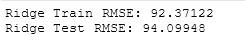
For the Ridge Regression Model, Train Root Mean Square Error came out to be 92.37 while Test Root Mean Square Error came out to be 94.09. As
discussed earlier, a perfect model often shows almost equal Train and Test Errors. We will compare this difference of these Error terms with the Classical Regression Model and the rest of Regularized Regression Models.
3. ElasticNet Regression
ElasticNet Regression is based on both L1 and L2 Regularization techniques. In ElasticNet regression, both L1 and L2 penalties are added to the cost function. Learn more about the ElasticNet Regression on Analytics Vidhya and here.
Now, let’s build an ElasticNet Regression Model and evaluate the RMSE for Train and Test Set.
Importing the libraries
import numpy as np
import pandas as pd
from sklearn.model_selection import train_test_split
from sklearn.linear_model import ElasticNet
from sklearn import metrics
import warnings
warnings.filterwarnings('ignore')
Importing the Dataset
df = pd.read_csv('Fish.csv')
The dataset has been taken from Kaggle
Specifying the x and y variables
x = df.drop('Weight', axis = 1)
y = df['Weight']
y = y.values.reshape(-1,1)
For this dataset, our task is to predict the Weight of the Fishes based on several features. Thus, ‘Weight‘ is our target feature. For the x
variable, we are taking every feature except the target variable
‘Weight’ and for y variable, we are taking just the target ‘Weight‘.
Creating Dummies for Categorical Variables
x = pd.get_dummies(x, drop_first = True)
Since our dataset contains a categorical feature, we will use the .get_dummies() method of pandas to create dummies for the unique classes of the categorical feature. Set the drop_first parameter value to True,
to save ourselves from the dummy variable trap.
Creating Train and Test Sets
x_train, x_test, y_train, y_test = train_test_split(x, y, test_size = 0.3, random_state = 66)
Creating train and test sets for x and y variables using train_test_split module
Building a Lasso Regression Model
enet = ElasticNet()
Here we created an object enet for the module ElasticNet from the sklearn library.
Fitting Model with x and y train sets
enet.fit(x_train, y_train)
Calculating ElasticNet Train and Test Set RMSE
print("ElasticNet Train RMSE:", np.round(np.sqrt(metrics.mean_squared_error(y_train, enet.predict(x_train))), 5))
print("ElasticNet Test RMSE:", np.round(np.sqrt(metrics.mean_squared_error(y_test, enet.predict(x_test))), 5))
We are using the mean_squared_error method of the metrics module from the sklearn library. It takes the actual y and the predicted y arguments. For the Train RMSE, we used y_train as the actual y value and enet.predict(x_train) method for the predicted y value. For the Test RMSE, we used y_test as the actual y value and enet.predict(x_test) method for the predicted y value. The .predict() method of ElasticNet predicts the y value for the given x values (here x_train and x_test).
Putting it all together
import numpy as np
import pandas as pd
from sklearn.model_selection import train_test_split
from sklearn.linear_model import ElasticNet
from sklearn import metrics
import warnings
warnings.filterwarnings('ignore')
df = pd.read_csv('Fish.csv')
x = df.drop('Weight', axis = 1)
y = df['Weight']
y = y.values.reshape(-1,1)
x = pd.get_dummies(x, drop_first = True)
x_train, x_test, y_train, y_test = train_test_split(x, y, test_size = 0.3, random_state = 66)
enet = ElasticNet()
enet.fit(x_train, y_train)
print("ElasticNet Train RMSE:", np.round(np.sqrt(metrics.mean_squared_error(y_train, enet.predict(x_train))), 5))
print("ElasticNet Test RMSE:", np.round(np.sqrt(metrics.mean_squared_error(y_test, enet.predict(x_test))), 5))
On executing this, we get:
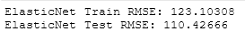
For the ElasticNet Regression Model, Train Root Mean Square Error came out to be 123.10 while Test Root Mean Square Error came out to be 110.42. As discussed earlier, a perfect model often shows almost equal Train and Test Errors. We will compare this difference of these Error terms with the Classical Regression Model and the rest of Regularized Regression Models.
Thus, based on the RMSE scores of Train and Test Sets of Regression Models built above, Ridge Regression Model performed the best as its
Train and test RMSE Score does not have a huge difference comparing with other built models.
Conclusions
In this article, we compared Reglairzed and Unregularized Multilinear Regression Models and compared their performances using Train and test sets RMSE scores. For the user data, the Ridge Regression Model performed best among the four models having almost equal RMSE scores. A good model generally has almost equal error values which is the case with RIdge Model here. One can try comparing the performances with different datasets of regression problems. Often we might need to scale the data, if required, to improve the performances. By default, the alpha value is set to 1. We can also try GridSearchCV or LassoCV / RidgeCV / ElasticNetCV to find the optimum value of alpha. One can try experimenting with more hyperparameters as the best way to learn is by doing.
About the Author
Connect with me on LinkedIn.
Check out my other Articles Here and on Medium
You can provide your valuable feedback to me on LinkedIn.
Thanks for giving your time!
IT Engineering Graduate currently pursuing Post Graduate Diploma in Data Science.


