Univariate Time Series Anomaly Detection Using ARIMA Model

This article was published as a part of the Data Science Blogathon

Anomaly Detection

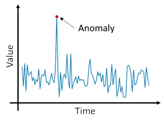
Anomaly detection is the process of finding anomalies in the data. Anomalies are the data points that deviate significantly from the general behaviour of the data. Detecting anomalies in the data can be much useful before training. Some examples of anomaly detection are Fraud detection, Spam filtering, CPU usage anomaly detection, Detecting anomalies in the server usage, and etc.

Time Series Data

The observations in the data are associated with a timestamp in time series data. The data is sequentially placed, so we can’t shuffle the data during training. The observations in the data are autocorrelated, which means the observations are highly related to their previous observations. The time-series data must be handled in a special way due to these constraints.

Time Series Anomaly Detection

To detect anomalies in the time series data, we can’t use the traditional anomaly detection algorithms like IQR, Isolation Forest, COPOD, and etc. We need to handle the task of time series anomaly detection in a separate way.

Steps to be followed to find anomalies in time-series data,

1. Check whether the data is stationary or not. If the data is not stationary convert the data to stationary.
2. Fit a time series model to the preprocessed data
3. Find the Squared Error for each and every observation in the data.
4. Find the threshold for the errors in the data
5. If the errors exceed that threshold we can flag that observation as an anomaly

Why do we use this approach?

As mentioned earlier, the time-series data is strictly sequential and is highly prone to autocorrelation. The time-series models would use the data to train and find the general behaviour of the data and tries to forecast the data. If an observation is normal the forecast would be as close as possible to the actual value, if an observation is an anomaly the forecast would be as far as possible to the actual value, so if we examine the errors of the forecast we could find the anomalies in the data.

Univariate vs. Multivariate Time Series Data

• Univariate time-series data would contain only one feature (or column) and a timestamp column associated with it.
• Multivariate time-series data would contain more than one feature and a timestamp column associated with it.

In this post, we are going to see about univariate time series anomaly detection.

Univariate Time Series Anomaly Detection

We are going to use the Air Passengers’ data from Kaggle. You can find the data here. The data contains the number of passengers boarded on an aeroplane per month. The data contains two columns, month and number of passengers.

def test_stationarity(ts_data, column='', signif=0.05, series=False):
    if series:
        adf_test = adfuller(ts_data, autolag='AIC')
    else:
        adf_test = adfuller(ts_data[column], autolag='AIC')
    p_value = adf_test[1]
    if p_value <= signif:
        test_result = "Stationary"
    else:
        test_result = "Non-Stationary"
    return test_result

"""Univariate Time Series"""

First of all, we are going to check whether the data is stationary or not using the Augmented Dickey-Fuller (ADF) test. The test would show us whether the data is stationary or not.

The ADF test returns the stats, which contain the p-value in it. The p-value is used to determine whether the data is stationary or not. If the p-value is less than 0.05 then the data is stationary or if the data is greater than 0.05 then the data is non-stationary. The 0.05 is called the significance level which corresponds to 95%. You can also try out different significance levels to test stationarity.

test_stationarity(data, 'Passengers') # Output: Non-Stationary

The test results show us that the data is non-stationary, which means the data doesn’t have constant mean, variance, and autocorrelation. To convert the data into stationary we can do differencing for the data.

def differencing(data, column, order):
    differenced_data = data[column].diff(order)
    differenced_data.fillna(differenced_data.mean(), inplace=True)
    return differenced_data
preprocessed_data = differencing(data, 'Passengers', 1)

The above code will difference the data which makes the data stationary. Let’s now check whether the differenced data is stationary or not using the ADF test.

test_stationarity(preprocessed_data, series=True) # Output: Stationary

After differencing the data has become stationary. Now we can use this data to train the time series model.

Here, we are going to use ARMA (AutoRegressive Moving Average) model to forecast the data. The ARMA model has two parameters namely p and q. The p is for the AR (Auto Regression) and the q is for MA (Moving Average). The Auto Regression uses the previous lags to model the data and the Moving Average uses the previous forecast errors to model the data.

The Auto Regression uses the lags of the data as features and the provided data as the target and uses the Least-squares method (or linear regression) to model the relationship between the data. As mentioned earlier we are using this to model time-series data which is strictly sequential and has autocorrelation. We can’t use least-squares or linear regression directly here because of the autocorrelation of the residuals. The autocorrelation of the residuals would result in spurious predictions. That is why we use a special model constructed specially for time-series data.

To find the best order (p, q ) for the model we have to select the order (p, q) that reduces the AIC for the model. We can find that using the following code.

max_p, max_q = 5, 5 
def get_order_sets(n, n_per_set) -> list:
    n_sets = [i for i in range(n)]
    order_sets = [
        n_sets[i:i + n_per_set]
        for i in range(0, n, n_per_set)
    ]
    return order_sets
def find_aic_for_model(data, p, q, model, model_name):
    try:
        msg = f"Fitting {model_name} with order p, q = {p, q}n"
        print(msg)
        if p == 0 and q == 1:
            # since p=0 and q=1 is already
            # calculated
            return None, (p, q)
        ts_results = model(data, order=(p, q)).fit(disp=False)
        curr_aic = ts_results.aic
        return curr_aic, (p, q)
    except Exception as e:
        f"""Exception occurred continuing {e}"""
        return None, (p, q)
def find_best_order_for_model(data, model, model_name):
    p_ar, q_ma = max_p, max_q
    final_results = []
    ts_results = model(data, order=(0, 1)).fit(disp=False)
    min_aic = ts_results.aic
    final_results.append((min_aic, (0, 1)))
    # example if q_ma is 6
    # order_sets would be [[0, 1, 2, 3, 4], [5]]
    order_sets = get_order_sets(q_ma, 5)
    for p in range(0, p_ar):
        for order_set in order_sets:
            # fit the model and find the aic
            results = Parallel(n_jobs=len(order_set), prefer='threads')(
                delayed(find_aic_for_model)(data, p, q, model, model_name)
                for q in order_set
            )
            final_results.extend(results)
    results_df = pd.DataFrame(
        final_results,
        columns=['aic', 'order']
    )
    min_df = results_df[
        results_df['aic'] == results_df['aic'].min()
    ]
    min_aic = min_df['aic'].iloc[0]
    min_order = min_df['order'].iloc[0]
    return min_aic, min_order, results_df
min_aic, min_order, results_df = find_best_order_for_model(
    preprocessed_data, ARMA, "ARMA"
)
print(min_aic, min_order)# Output: 1341.1035677173795, (4, 4)

How does the above code work?

• We should provide the maximum values for p and q to explore.
• The code above will fit the model for different p and q values and record the AIC for each model.
  • Here, I have used multi-threading to execute the code faster.
• After completing the best order is found using the minimum AIC value for the model.

Now that we have found that (4, 4) is the best order we can use that to fit the ARMA model.

def find_anomalies(squared_errors):
    threshold = np.mean(squared_errors) + np.std(squared_errors)
    predictions = (squared_errors >= threshold).astype(int)
    return predictions, threshold

arma = ARMA(preprocessed_data, order=min_order)
arma_fit = arma.fit()
squared_errors = arma_fit.resid ** 2
predictions, threshold = find_anomalies(squared_errors) # threshold = 1428.0094261298002

We are fitting the model with (4, 4) order. The resid attribute of the fitted results will have the residuals of each observation and forecast.

We are using the following formula to find the threshold for the squared errors above which the data is considered to be an anomaly.

threshold = mean(squared_errors) + (z * standard_deviation(squared_errors))

z is an integer. Here we have used z=1. You can adjust the value of z to obtain different thresholds according to your needs. There are other methods to find the threshold like finding the 90th percentile of the errors. This method could also be used to find the threshold.

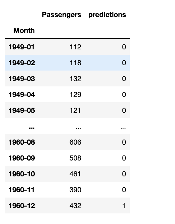
The predictions will contain the integers 0 and 1 which indicate normal and anomalous observations respectively.

data['predictions'] = predictions
print(data)

Summary

• Find whether the data is stationary or not.
• Convert the data to stationary if it is not stationary using differencing
• Find the best order for the ARMA model
• Fit the ARMA model and find the squared errors
• Find the threshold using squared errors
• The errors above the threshold are considered to be anomalous data.

Srivignesh R 09 Sep 2022

Machine Learning Engineer @ Zoho Corporation