10 Automated Machine Learning for Supervised Learning (Part 2)
This article was published as a part of the Data Science Blogathon
Introduction
This post will discuss 10 Automated Machine Learning (autoML) packages that we can run in Python. If you are tired of running lots of Machine Learning algorithms just to find the best one, this post might be what you are looking for. This post is the second part of this first post. The first part explains the general concept of Machine Learning from defining the objective, pre-processing, model creation and selection, hyperparameter-tuning, and model evaluation. At the end of that post, Auto-Sklearn is introduced as an autoML. If you are already familiar with Machine Learning, you can skip that part 1.
The main point of the first part is that we require a relatively long time and many lines of code to run all of the classification or regression algorithms before finally selecting or ensembling the best models. Instead, we can run AutoML to automatically search for the best model with a much shorter time and, of course, less code. Please find my notebooks for conventional Machine Learning algorithms for regression (predicting house prices) and classification (predicting poverty level classes) tasks in the table below. My AutoML notebooks are also in the table below. Note that this post will focus only on regression and classification AutoML while AutoML also can be applied for image, NLP or text, and time series forecasting.
| Regression | Classification | |
| Conventional Machine Learning | Conventional Regression | Conventional Classification |
| Automated Machine Learning | Part 1, Part 2 | Part 1, Part 2 |
Now, we will start discussing the 10 AutoML packages that can replace those long notebooks.
AutoSklearn
This autoML, as mentioned above, has been discussed before. Let’s do a quick recap. Below is the code for searching for the best model in 3 minutes. More details are explained in the first part.
Regression
!apt install -y build-essential swig curl
!curl https://raw.githubusercontent.com/automl/auto-sklearn/master/requirements.txt | xargs -n 1 -L 1 pip install
!pip install auto-sklearn
!pip install scipy==1.7.0
!pip install -U scikit-learn
from autosklearn.regression import AutoSklearnRegressor
from sklearn.metrics import mean_squared_error, mean_absolute_error
Running AutoSklearn
# Create the model
sklearn = AutoSklearnRegressor(time_left_for_this_task=3*60, per_run_time_limit=30, n_jobs=-1)
# Fit the training data
sklearn.fit(X_train, y_train)
# Sprint Statistics
print(sklearn.sprint_statistics())
# Predict the validation data
pred_sklearn = sklearn.predict(X_val)
# Compute the RMSE
rmse_sklearn=MSE(y_val, pred_sklearn)**0.5
print('RMSE: ' + str(rmse_sklearn))
Output:
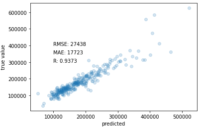
auto-sklearn results:
   Dataset name: c40b5794-fa4a-11eb-8116-0242ac130202
   Metric: r2
   Best validation score: 0.888788
   Number of target algorithm runs: 37
   Number of successful target algorithm runs: 23
   Number of crashed target algorithm runs: 0
   Number of target algorithms that exceeded the time limit: 8
   Number of target algorithms that exceeded the memory limit: 6
 RMSE: 27437.715258009852
Result:
# Scatter plot true and
predicted values
plt.scatter(pred_sklearn, y_val, alpha=0.2)
plt.xlabel('predicted')
plt.ylabel('true value')
plt.text(100000, 400000, 'RMSE: ' + str(round(rmse_sklearn)))
plt.text(100000, 350000, 'MAE: ' + str(round(mean_absolute_error(y_val,
pred_sklearn))))
plt.text(100000, 300000, 'R: ' + str(round(np.corrcoef(y_val,
pred_sklearn)[0,1],4)))
plt.show()
Classification
Applying AutoML
!apt install -y build-essential swig curl
!curl https://raw.githubusercontent.com/automl/auto-sklearn/master/requirements.txt | xargs -n 1 -L 1 pip install
from autosklearn.classification import AutoSklearnClassifier
# Create the model
sklearn = AutoSklearnClassifier(time_left_for_this_task=3*60, per_run_time_limit=15, n_jobs=-1)
# Fit the training data
sklearn.fit(X_train, y_train)
# Sprint Statistics
print(sklearn.sprint_statistics())
# Predict the validation data
pred_sklearn = sklearn.predict(X_val)
# Compute the accuracy
print('Accuracy: ' + str(accuracy_score(y_val, pred_sklearn)))
Output:
auto-sklearn results:
   Dataset name: 576d4f50-c85b-11eb-802c-0242ac130202
   Metric: accuracy
   Best validation score: 0.917922
   Number of target algorithm runs: 40
   Number of successful target algorithm runs: 8
   Number of crashed target algorithm runs: 0
   Number of target algorithms that exceeded the time limit: 28
   Number of target algorithms that exceeded the memory limit: 4
 Accuracy: 0.923600209314495
Result:
# Prediction results
print('Confusion Matrix')
print(pd.DataFrame(confusion_matrix(y_val, pred_sklearn), index=[1,2,3,4], columns=[1,2,3,4]))
print('')
print('Classification Report')
print(classification_report(y_val, pred_sklearn))
Output:
Confusion Matrix
     1    2    3     4
1  123   14    3    11
2   17  273   11    18
3    3   17  195    27
4    5   15    5  1174
Classification Report
              precision    recall  f1-score   support
           1       0.83      0.81      0.82       151
           2       0.86      0.86      0.86       319
           3       0.91      0.81      0.86       242
           4       0.95      0.98      0.97      1199
    accuracy                           0.92      1911
   macro avg       0.89      0.86      0.88      1911
weighted avg       0.92      0.92      0.92      1911
Tree-based Pipeline Optimization Tool (TPOT)
TPOT is built on top of scikit-learn. TPOT uses a genetic algorithm to search for the best model according to the “generations” and “population size”. The higher the two parameters are set, the longer will it take time. Unlike AutoSklearn, we do not set the specific running time for TPOT. As its name suggests, after the TPOT is run, it exports lines of code containing a pipeline from importing packages, splitting the dataset, creating the tuned model, fitting the model, and finally predicting the validation dataset. The pipeline is exported in .py format.
In the code below, I set the generation and population_size to be 5. The output gives 5 generations with increasing “scoring”. I set the scoring to be “neg_mean_absolute_error” and” accuracy” for regression and classification tasks respectively. Neg_mean_absolute_error means Mean Absolute Error (MAE) in negative form. The algorithm chooses the highest scoring value. Making the MAE negative will make the algorithm selecting the MAE closest to zero.
Regression
from tpot import TPOTRegressor
# Create model
cv = RepeatedStratifiedKFold(n_splits=3, n_repeats=3, random_state=123)
tpot = TPOTRegressor(generations=5, population_size=5, cv=cv, scoring='neg_mean_absolute_error', verbosity=2, random_state=123, n_jobs=-1)
# Fit the training data
tpot.fit(X_train, y_train)
# Export the result
tpot.export('tpot_model.py')
Output:
Generation 1 - Current best internal CV score: -20390.588131563232
Generation 2 - Current best internal CV score: -19654.82630417806
Generation 3 - Current best internal CV score: -19312.09139004322
Generation 4 - Current best internal CV score: -19312.09139004322
Generation 5 - Current best internal CV score: -18752.921100941825
Best pipeline: RandomForestRegressor(input_matrix, bootstrap=True, max_features=0.25, min_samples_leaf=3, min_samples_split=2, n_estimators=100)
Classification
from tpot import TPOTClassifier
# TPOT that are stopped earlier. It still gives temporary best pipeline.
# Create the model
cv = RepeatedStratifiedKFold(n_splits=3, n_repeats=3, random_state=123)
tpot = TPOTClassifier(generations=5, population_size=5, cv=cv, scoring='accuracy', verbosity=2, random_state=123, n_jobs=-1)
# Fit the training data
tpot.fit(X_train, y_train)
# Export the result
tpot.export('tpot_model.py')
Output:
Generation 1 - Current best internal CV score: 0.7432273262661955
Generation 2 - Current best internal CV score: 0.843824979278454
Generation 3 - Current best internal CV score: 0.8545565589146273
Generation 4 - Current best internal CV score: 0.8545565589146273
Generation 5 - Current best internal CV score: 0.859616978580465
Best pipeline: RandomForestClassifier(GradientBoostingClassifier(input_matrix, learning_rate=0.001, max_depth=2, max_features=0.7000000000000001, min_samples_leaf=1, min_samples_split=19, n_estimators=100, subsample=0.15000000000000002), bootstrap=True, criterion=gini, max_features=0.8500000000000001, min_samples_leaf=4, min_samples_split=12, n_estimators=100)
AutoSklearn gives the result of RandomForestRegressor for the regression task. As for the classification, it gives the stacking of GradientBoostingClassifier and RandomForestClassifier. All algorithms already have their hyperparameters tuned.
Here is to see the validation data scoring metrics.
Regression
pred_tpot = results
# Scatter plot true and predicted values
plt.scatter(pred_tpot, y_val, alpha=0.2)
plt.xlabel('predicted')
plt.ylabel('true value')
plt.text(100000, 400000, 'RMSE: ' + str(round(MSE(y_val, pred_tpot)**0.5)))
plt.text(100000, 350000, 'MAE: ' + str(round(mean_absolute_error(y_val, pred_tpot))))
plt.text(100000, 300000, 'R: ' + str(round(np.corrcoef(y_val, pred_tpot)[0,1],4)))
plt.show()
Output:
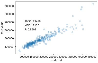
Fig. 2 TPOT regression result.
Classification
pred_tpot = results
# Compute the accuracy
print('Accuracy: ' + str(accuracy_score(y_val, pred_tpot)))
print('')
# Prediction results
print('Confusion Matrix')
print(pd.DataFrame(confusion_matrix(y_val, pred_tpot), index=[1,2,3,4], columns=[1,2,3,4]))
print('')
print('Classification Report')
print(classification_report(y_val, pred_tpot))
Output:
Accuracy: 0.9246467817896389

Confusion Matrix
     1    2    3     4
1  117   11    7    16
2    6  288   10    15
3    2   18  186    36
4    5   12    6  1176

Classification Report
              precision    recall  f1-score   support

           1       0.90      0.77      0.83       151
           2       0.88      0.90      0.89       319
           3       0.89      0.77      0.82       242
           4       0.95      0.98      0.96      1199

    accuracy                           0.92      1911
   macro avg       0.90      0.86      0.88      1911
weighted avg       0.92      0.92      0.92      1911
Distributed Asynchronous Hyper-parameter Optimization (Hyperopt)
Hyperopt is also usually used to optimize the hyperparameters of one model that has been specified. For example, we decide to apply Random Forest and then run hyperopt to find the optimal hyperparameters for the Random Forest. My previous post discussed it. But, this post is different in that it uses hyperopt to search for the best Machine Learning model automatically, not just tuning the hyperparameters. The code is similar but different.
The code below shows how to use hyperopt to run AutoML. Max evaluation of 50 and trial timeout of 20 seconds is set. These will determine how long the AutoML will work. Like in TPOT, we do not set the time limit in hyperopt.
Regression
!pip install git+https://github.com/hyperopt/hyperopt-sklearn.git
from hpsklearn import HyperoptEstimator
from hpsklearn import any_regressor
from hpsklearn import any_preprocessing
from hyperopt import tpe
from sklearn.metrics import mean_squared_error
# Create the model
hyperopt = HyperoptEstimator(regressor=any_regressor('reg'), preprocessing=any_preprocessing('pre'),
                             loss_fn=mean_squared_error, algo=tpe.suggest, max_evals=50,
                             trial_timeout=20)
# Fit the data
hyperopt.fit(X_train, y_train)
Classification
!pip install git+https://github.com/hyperopt/hyperopt-sklearn.git
from hpsklearn import HyperoptEstimator
from hpsklearn import any_classifier
from hpsklearn import any_preprocessing
from hyperopt import tpe
# Create the model
hyperopt = HyperoptEstimator(classifier=any_classifier('cla'), preprocessing=any_preprocessing('pre'),
                             algo=tpe.suggest, max_evals=50, trial_timeout=30)
# Fit the training data
hyperopt.fit(X_train_ar, y_train_ar)
In the Kaggle notebook (in the table above), every time I finished performing the fitting and predicting, I will show the prediction of validation data results in scatter plot, confusion matrix, and classification report. The code is always almost the same with a little adjustment. So, from this point onwards, I am not going to put them in this post. But, the Kaggle notebook provides them.
To see the algorithm from the AutoML search result. Use the below code. The results are ExtraTreeClassfier and XGBRegressor. Observe that it also searches for the preprocessing technics, such as standard scaler and normalizer.
# Show the models
print(hyperopt.best_model())
Regression
{'learner': XGBRegressor(base_score=0.5, booster='gbtree',
            colsample_bylevel=0.6209369845565308, colsample_bynode=1,
            colsample_bytree=0.6350745975782562, gamma=0.07330922089021298,
            gpu_id=-1, importance_type='gain', interaction_constraints='',
            learning_rate=0.0040826994703554555, max_delta_step=0,
            max_depth=10, min_child_weight=1, missing=nan,
            monotone_constraints='()', n_estimators=2600, n_jobs=1,
            num_parallel_tree=1, objective='reg:linear', random_state=3,
            reg_alpha=0.4669165283261672, reg_lambda=2.2280355282357056,
            scale_pos_weight=1, seed=3, subsample=0.7295609371405459,
            tree_method='exact', validate_parameters=1, verbosity=None), 'preprocs': (Normalizer(norm='l1'),), 'ex_preprocs': ()}
Classification
{'learner': ExtraTreesClassifier(bootstrap=True, max_features='sqrt', n_estimators=308,
                    n_jobs=1, random_state=1, verbose=False), 'preprocs': (StandardScaler(with_std=False),), 'ex_preprocs': ()}
AutoKeras
AutoKeras, as you might guess, is an autoML specializing in Deep Learning or Neural networks. The “Keras” in the name gives the clue. AutoKeras helps in finding the best neural network architecture and hyperparameters for the prediction model. Unlike the other AutoML, AutoKeras does not consider tree-based, distance-based, or other Machine Learning algorithms.
Deep Learning is challenging not only for the hyperparameter-tuning but also for the architecture setting. Many ask about how many neurons or layers are the best to use. There is no clear answer to that. Conventionally, users must try to run and evaluate their Deep Learning architectures one by one before finally decide which one is the best. It takes a long time and resources to accomplish. I wrote a post describing this here. However, AutoKeras can solve this problem.
To apply the AutoKeras, I set the max_trials to be 8 and it will try to find the best deep learning architecture for a maximum of 8 trials. Set the epoch while fitting the training dataset and it will determine the accuracy of the model.
Regression
!pip install autokeras
import autokeras
# Create the model
keras = autokeras.StructuredDataRegressor(max_trials=8)
# Fit the training dataset
keras.fit(X_train, y_train, epochs=100)
# Predict the validation data
pred_keras = keras.predict(X_val)
Classification
!pip install autokeras
import autokeras
# Create the model
keras = autokeras.StructuredDataClassifier(max_trials=8)
# Fit the training dataset
keras.fit(X_train, y_train, epochs=100)
# Predict the validation data
pred_keras = keras.predict(X_val)
# Compute the accuracy
print('Accuracy: ' + str(accuracy_score(y_val, pred_keras)))
To find the architecture of the AutoKeras search, use the following code.
# Show the built models
keras_export = keras.export_model()
keras_export.summary()
Regression
Model: "model"
 _________________________________________________________________
 Layer (type)                 Output Shape              Param #
 =================================================================
 input_1 (InputLayer)         [(None, 20)]              0
 _________________________________________________________________
 multi_category_encoding (Mul (None, 20)                0
 _________________________________________________________________
 dense (Dense)                (None, 512)               10752
 _________________________________________________________________
 re_lu (ReLU)                 (None, 512)               0
 _________________________________________________________________
 dense_1 (Dense)              (None, 32)                16416
 _________________________________________________________________
 re_lu_1 (ReLU)               (None, 32)                0
 _________________________________________________________________
 regression_head_1 (Dense)    (None, 1)                 33
 =================================================================
 Total params: 27,201
 Trainable params: 27,201
 Non-trainable params: 0
 _________________________________________________________________
Classification
Model: "model"
 _________________________________________________________________
 Layer (type)                 Output Shape              Param #
 =================================================================
 input_1 (InputLayer)         [(None, 71)]              0
 _________________________________________________________________
 multi_category_encoding (Mul (None, 71)                0
 _________________________________________________________________
 normalization (Normalization (None, 71)                143
 _________________________________________________________________
 dense (Dense)                (None, 512)               36864
 _________________________________________________________________
 re_lu (ReLU)                 (None, 512)               0
 _________________________________________________________________
 dense_1 (Dense)              (None, 32)                16416
 _________________________________________________________________
 re_lu_1 (ReLU)               (None, 32)                0
 _________________________________________________________________
 dropout (Dropout)            (None, 32)                0
 _________________________________________________________________
 dense_2 (Dense)              (None, 4)                 132
 _________________________________________________________________
 classification_head_1 (Softm (None, 4)                 0
 =================================================================
 Total params: 53,555
 Trainable params: 53,412
 Non-trainable params: 143
 _________________________________________________________________
MLJAR
MLJAR is another great AutoML. And, you will find why soon. To run MLJAR, I assign the arguments of mode, eval_metric, total_time_limit, and feature_selection. This AutoML will understand whether it is a regression or classification task from the eval_metric. The total_time_limit is the duration of how long we allow MLJAR to run in seconds. In this case, it will take 300 seconds or 5 minutes to find the possible best model. We can also specify whether to allow feature selection. The output then will report the used algorithms and how long they take to finish.
Regression
!pip install -q -U git+https://github.com/mljar/mljar-supervised.git@master
from supervised.automl import AutoML
# Create the model
mljar = AutoML(mode="Compete",  eval_metric="rmse", total_time_limit=300,
               features_selection=True)
# Fit the training data
mljar.fit(X_train, y_train)
# Predict the training data
mljar_pred = mljar.predict(X_val)
Classification
!pip install -q -U git+https://github.com/mljar/mljar-supervised.git@master
from supervised.automl import AutoML
# Create the model
mljar = AutoML(mode="Compete",  eval_metric="accuracy", total_time_limit=300,
               features_selection=True)
# Fit the training data
mljar.fit(X_train, y_train)
# Predict the training data
mljar_pred = mljar.predict(X_val)
The argument “mode” lets us decide what the MLJAR is expected for. There are 4 types of modes to define the purpose of running the MLJAR. In the example code above, the mode of “compete” is used for winning a competition by finding the best model by tuning and ensembling methods. The mode of “optuna” is used to find the best-tuned model with unlimited computation time. The mode of “perform” builds a Machine Learning pipeline for production. The mode of “explain” is used for data explanation.
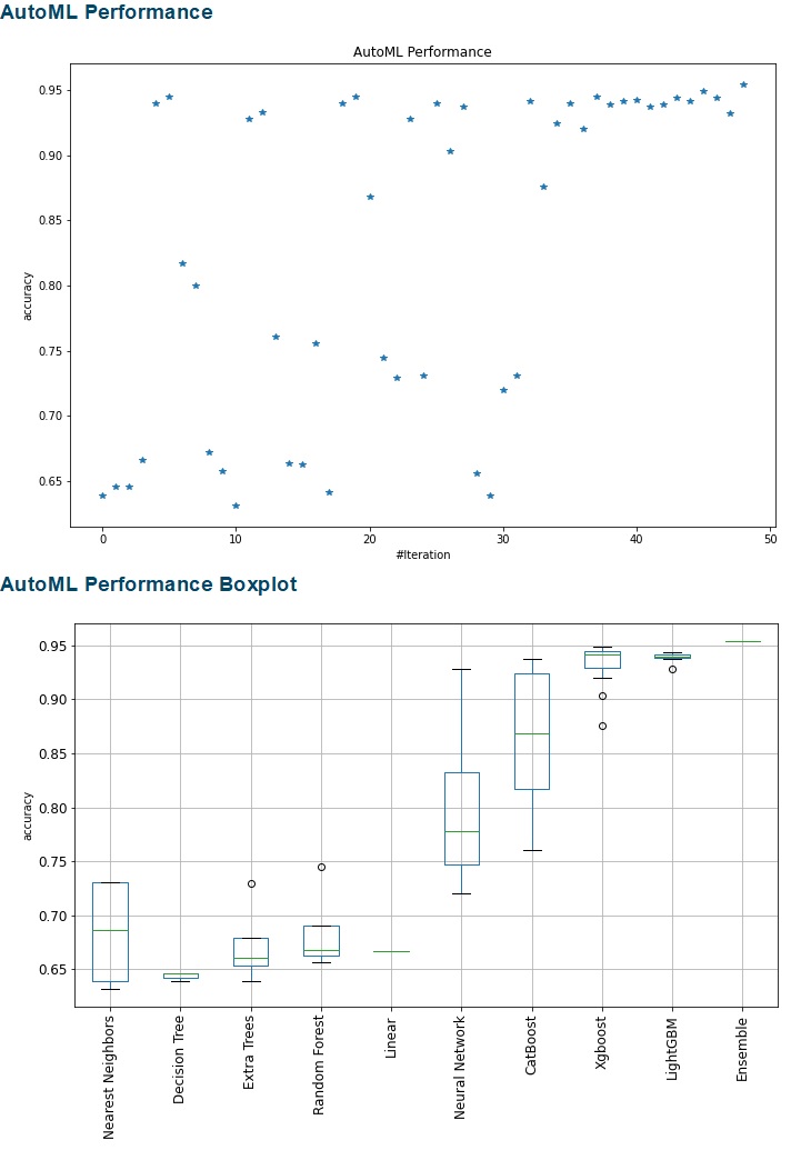
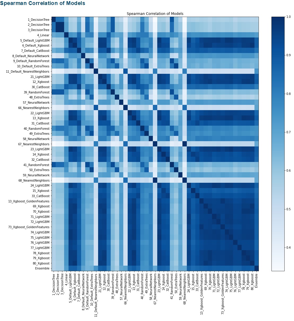
The result of MLJAR is automatically reported and visualized. Unfortunately, Kaggle does not display the report result after saving. So, below is how it should look. The report compares the MLJAR results for every algorithm. We can see the ensemble methods have the lowest MSE for the regression task and the highest accuracy for the classification task. The increasing number of iteration lowers the MSE for the regression task and improves the accuracy of the classification task. (The leaderboard tables below actually have more rows, but they were cut.)
Regression
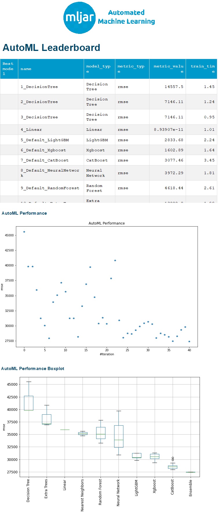
Fig. 3 MLJAR Report for regression
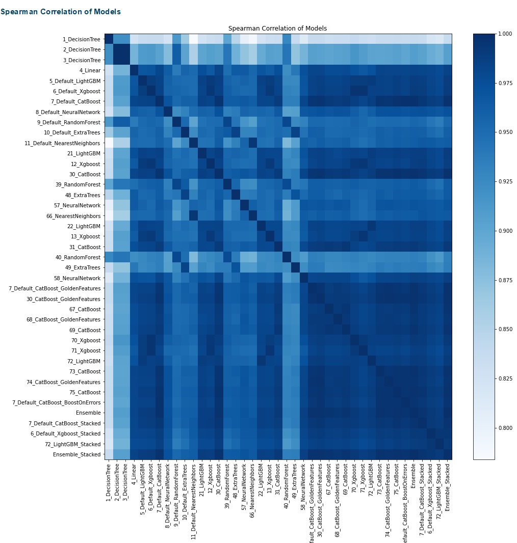
Fig. 4 MLJAR for regession
AutoGluon
AutoGluon requires users to format the training dataset using TabularDataset to recognize it. Users can then specify the time_limit allocation for AutoGluon to work. In the example code below, I set it to be 120 seconds or 2 minutes.
Regression
!pip install -U pip
!pip install -U setuptools wheel
!pip install -U "mxnet<2.0.0"
!pip install autogluon
from autogluon.tabular import TabularDataset, TabularPredictor
# Prepare the data
Xy_train = X_train.reset_index(drop=True)
Xy_train['Target'] = y_train
Xy_val = X_val.reset_index(drop=True)
Xy_val['Target'] = y_val
X_train_gluon = TabularDataset(Xy_train)
X_val_gluon = TabularDataset(Xy_val)
# Fit the training data
gluon = TabularPredictor(label='Target').fit(X_train_gluon, time_limit=120)
# Predict the training data
gluon_pred = gluon.predict(X_val)
Classification
!pip install -U pip
!pip install -U setuptools wheel
!pip install -U "mxnet<2.0.0"
!pip install autogluon
from autogluon.tabular import TabularDataset, TabularPredictor
# Prepare the data
Xy_train = X_train.reset_index(drop=True)
Xy_train['Target'] = y_train
Xy_val = X_val.reset_index(drop=True)
Xy_val['Target'] = y_val
X_train_gluon = TabularDataset(Xy_train)
X_val_gluon = TabularDataset(Xy_val)
# Fit the training data
gluon = TabularPredictor(label='Target').fit(X_train_gluon, time_limit=120)
# Predict the training data
gluon_pred = gluon.predict(X_val)
After finishing the task, AutoGluon can report the accuracy of each Machine Learning algorithm it has tried. The report is called leaderboard. The columns below are actually longer, but I cut them for this post.
# Show the models
leaderboard = gluon.leaderboard(X_train_gluon)
leaderboard
Regression
| model | score_test | score_val | pred_time_test | . . . | |
| 0 | RandomForestMSE | -15385.131260 | -23892.159881 | 0.133275 | . . . |
| 1 | ExtraTreesMSE | -15537.139720 | -24981.601931 | 0.137063 | . . . |
| 2 | LightGBMLarge | -17049.125557 | -26269.841824 | 0.026560 | . . . |
| 3 | XGBoost | -18142.996982 | -23573.451829 | 0.054067 | . . . |
| 4 | KNeighborsDist | -18418.785860 | -41132.826848 | 0.135036 | . . . |
| 5 | CatBoost | -19585.309377 | -23910.403833 | 0.004854 | . . . |
| 6 | WeightedEnsemble_L2 | -20846.144676 | -22060.013365 | 1.169406 | . . . |
| 7 | LightGBM | -23615.121228 | -23205.065207 | 0.024396 | . . . |
| 8 | LightGBMXT | -25261.893395 | -24608.580984 | 0.015091 | . . . |
| 9 | NeuralNetMXNet | -28904.712029 | -24104.217749 | 0.819149 | . . . |
| 10 | KNeighborsUnif | -39243.784302 | -39545.869493 | 0.132839 | . . . |
| 11 | NeuralNetFastAI | -197411.475391 | -191261.448480 | 0.070965 | . . . |
Classification
| model | score_test | score_val | pred_time_test | . . . | |
| 0 | WeightedEnsemble_L2 | 0.986651 | 0.963399 | 3.470253 | . . . |
| 1 | LightGBM | 0.985997 | 0.958170 | 0.600316 | . . . |
| 2 | XGBoost | 0.985997 | 0.956863 | 0.920570 | . . . |
| 3 | RandomForestEntr | 0.985866 | 0.954248 | 0.366476 | . . . |
| 4 | RandomForestGini | 0.985735 | 0.952941 | 0.397669 | . . . |
| 5 | ExtraTreesEntr | 0.985735 | 0.952941 | 0.398659 | . . . |
| 6 | ExtraTreesGini | 0.985735 | 0.952941 | 0.408386 | . . . |
| 7 | KNeighborsDist | 0.985473 | 0.950327 | 2.013774 | . . . |
| 8 | LightGBMXT | 0.984034 | 0.951634 | 0.683871 | . . . |
| 9 | NeuralNetFastAI | 0.983379 | 0.947712 | 0.340936 | . . . |
| 10 | NeuralNetMXNet | 0.982332 | 0.956863 | 2.459954 | . . . |
| 11 | CatBoost | 0.976574 | 0.934641 | 0.044412 | . . . |
| 12 | KNeighborsUnif | 0.881560 | 0.769935 | 1.970972 | . . . |
| 13 | LightGBMLarge | 0.627143 | 0.627451 | 0.014708 | . . . |
H2O
Similar to AutoGluon, H2O requires the training dataset in a certain format, called H2OFrame. To decide how long H2O will work, either max_runtime_secs or max_models must be specified. The names explain what they mean.
Regression
import h2o
from h2o.automl import H2OAutoML
h2o.init()
# Prepare the data
Xy_train = X_train.reset_index(drop=True)
Xy_train['SalePrice'] = y_train.reset_index(drop=True)
Xy_val = X_val.reset_index(drop=True)
Xy_val['SalePrice'] = y_val.reset_index(drop=True)
# Convert H2O Frame
Xy_train_h2o = h2o.H2OFrame(Xy_train)
X_val_h2o = h2o.H2OFrame(X_val)
# Create the model
h2o_model = H2OAutoML(max_runtime_secs=120, seed=123)
# Fit the model
h2o_model.train(x=Xy_train_h2o.columns, y='SalePrice', training_frame=Xy_train_h2o)
# Predict the training data
h2o_pred = h2o_model.predict(X_val_h2o)
Classification
import h2o
from h2o.automl import H2OAutoML
h2o.init()
# Convert H2O Frame
Xy_train_h2o = h2o.H2OFrame(Xy_train)
X_val_h2o = h2o.H2OFrame(X_val)
Xy_train_h2o['Target'] = Xy_train_h2o['Target'].asfactor()
# Create the model
h2o_model = H2OAutoML(max_runtime_secs=120, seed=123)
# Fit the model
h2o_model.train(x=Xy_train_h2o.columns, y='Target', training_frame=Xy_train_h2o)
# Predict the training data
h2o_pred = h2o_model.predict(X_val_h2o)
h2o_pred
For the classification task, the prediction result is a multilabel classification result. It gives the probability value for each class. Below is an example of the classification.
| predict | p1 | p2 | p3 | p4 |
| 4 | 0.0078267 | 0.0217498 | 0.0175197 | 0.952904 |
| 4 | 0.00190617 | 0.00130162 | 0.00116375 | 0.995628 |
| 4 | 0.00548938 | 0.0156449 | 0.00867845 | 0.970187 |
| 3 | 0.00484961 | 0.0161661 | 0.970052 | 0.00893224 |
| 2 | 0.0283297 | 0.837641 | 0.0575789 | 0.0764503 |
| 3 | 0.00141621 | 0.0022694 | 0.992301 | 0.00401299 |
| 4 | 0.00805432 | 0.0300103 | 0.0551097 | 0.906826 |
H2O reports its result by a simple table showing various scoring metrics of each Machine Learning algorithm.
# Show the model results
leaderboard_h2o = h2o.automl.get_leaderboard(h2o_model, extra_columns = 'ALL')
leaderboard_h2o
Regression output:
| model_id | mean_residual_deviance | rmse | mse | mae | rmsle | … |
| GBM_grid__1_AutoML_20210811_022746_model_17 | 8.34855e+08 | 28893.9 | 8.34855e+08 | 18395.4 | 0.154829 | … |
| GBM_1_AutoML_20210811_022746 | 8.44991e+08 | 29068.7 | 8.44991e+08 | 17954.1 | 0.149824 | … |
| StackedEnsemble_BestOfFamily_AutoML_20210811_022746 | 8.53226e+08 | 29210 | 8.53226e+08 | 18046.8 | 0.149974 | … |
| GBM_grid__1_AutoML_20210811_022746_model_1 | 8.58066e+08 | 29292.8 | 8.58066e+08 | 17961.7 | 0.153238 | … |
| GBM_grid__1_AutoML_20210811_022746_model_2 | 8.91964e+08 | 29865.8 | 8.91964e+08 | 17871.9 | 0.1504 | … |
| GBM_grid__1_AutoML_20210811_022746_model_10 | 9.11731e+08 | 30194.9 | 9.11731e+08 | 18342.2 | 0.153421 | … |
| GBM_grid__1_AutoML_20210811_022746_model_21 | 9.21185e+08 | 30351 | 9.21185e+08 | 18493.5 | 0.15413 | … |
| GBM_grid__1_AutoML_20210811_022746_model_8 | 9.22497e+08 | 30372.6 | 9.22497e+08 | 19124 | 0.159135 | … |
| GBM_grid__1_AutoML_20210811_022746_model_23 | 9.22655e+08 | 30375.2 | 9.22655e+08 | 17876.6 | 0.150722 | … |
| XGBoost_3_AutoML_20210811_022746 | 9.31315e+08 | 30517.5 | 9.31315e+08 | 19171.1 | 0.157819 | … |
Classification
| model_id | mean_per_class_error | logloss | rmse | mse | … |
| StackedEnsemble_BestOfFamily_AutoML_20210608_143533 | 0.187252 | 0.330471 | 0.309248 | 0.0956343 | … |
| StackedEnsemble_AllModels_AutoML_20210608_143533 | 0.187268 | 0.331742 | 0.309836 | 0.0959986 | … |
| DRF_1_AutoML_20210608_143533 | 0.214386 | 4.05288 | 0.376788 | 0.141969 | … |
| GBM_grid__1_AutoML_20210608_143533_model_1 | 0.266931 | 0.528616 | 0.415268 | 0.172447 | … |
| XGBoost_grid__1_AutoML_20210608_143533_model_1 | 0.323726 | 0.511452 | 0.409528 | 0.167713 | … |
| GBM_4_AutoML_20210608_143533 | 0.368778 | 1.05257 | 0.645823 | 0.417088 | … |
| GBM_grid__1_AutoML_20210608_143533_model_2 | 0.434227 | 1.10232 | 0.663382 | 0.440075 | … |
| GBM_3_AutoML_20210608_143533 | 0.461059 | 1.08184 | 0.655701 | 0.429944 | … |
| GBM_2_AutoML_20210608_143533 | 0.481588 | 1.08175 | 0.654895 | 0.428887 | … |
| XGBoost_1_AutoML_20210608_143533 | 0.487381 | 1.05534 | 0.645005 | 0.416031 | … |
PyCaret
This is the longest AutoML code that this post is exploring. PyCaret does not need splitting the features (X_train) and label (y_train). So, the below code will only randomly split the training dataset into another training dataset and a validation dataset. Preprocessing, such as filling missing data or feature selection, is also not required. Then, we set up the PyCaret by assigning the data, target variable or label, numeric imputation method, categorical imputation method, whether to use normalization, whether to remove multicollinearity, etc.
Regression
!pip install pycaret
from pycaret.regression import *
# Generate random numbers
val_index = np.random.choice(range(trainSet.shape[0]), round(trainSet.shape[0]*0.2), replace=False)
# Split trainSet
trainSet1 = trainSet.drop(val_index)
trainSet2 = trainSet.iloc[val_index,:]
# Create the model
caret = setup(data = trainSet1, target='SalePrice', session_id=111,
              numeric_imputation='mean',  categorical_imputation='constant',
              normalize = True, combine_rare_levels = True, rare_level_threshold = 0.05,
              remove_multicollinearity = True, multicollinearity_threshold = 0.95)
Classification
!pip install pycaret
from pycaret.classification import *
# Generate random numbers
val_index = np.random.choice(range(trainSet.shape[0]), round(trainSet.shape[0]*0.2), replace=False)
# Split trainSet
trainSet1 = trainSet.drop(val_index)
trainSet2 = trainSet.iloc[val_index,:]
# Create the model
caret = setup(data = trainSet1, target='Target', session_id=123,
              numeric_imputation='mean',  categorical_imputation='constant',
              normalize = True, combine_rare_levels = True, rare_level_threshold = 0.05,
              remove_multicollinearity = True, multicollinearity_threshold = 0.95)
After that, we can run the PyCaret by specifying how many cross-validations folds we want. The PyCaret for regression gives several models sorting from the best scoring metrics. The top models are Bayesian Ridge, Huber Regressor, Orthogonal Matching Pursuit, Ridge Regression, and Passive-Aggressive Regressor. The scoring metrics are MAE, MSE, RMSE, R2, RMSLE, and MAPE. PyCaret for classification also gives several models. The top models are the Extra Trees Classifier, Random Forest Classifier, Decision Tree Classifier, Extreme Gradient Boosting, and Light Gradient Boosting Machine. The below tables are limited for their rows and columns. Find the complete tables in the Kaggle notebook.
# Show the models
caret_models = compare_models(fold=5)
| Model | MAE | MSE | RMSE | R2 | … | |
| br | Bayesian Ridge | 15940.2956 | 566705805.8954 | 23655.0027 | 0.9059 | … |
| huber | Huber Regressor | 15204.0960 | 588342119.6640 | 23988.3772 | 0.9033 | … |
| omp | Orthogonal Matching Pursuit | 16603.0485 | 599383228.9339 | 24383.2437 | 0.9001 | … |
| ridge | Ridge Regression | 16743.4660 | 605693331.2000 | 24543.6840 | 0.8984 | … |
| par | Passive Aggressive Regressor | 15629.1539 | 630122079.3113 | 24684.8617 | 0.8972 | … |
| … | … | … | … | … | … | … |
Classification
| Model | Accuracy | AUC | Recall | Prec. | … | |
| et | Extra Trees Classifier | 0.8944 | 0.9708 | 0.7912 | 0.8972 | … |
| rf | Random Forest Classifier | 0.8634 | 0.9599 | 0.7271 | 0.8709 | … |
| dt | Decision Tree Classifier | 0.8436 | 0.8689 | 0.7724 | 0.8448 | … |
| xgboost | Extreme Gradient Boosting | 0.8417 | 0.9455 | 0.7098 | 0.8368 | … |
| lightgbm | Light Gradient Boosting Machine | 0.8337 | 0.9433 | 0.6929 | 0.8294 | … |
| … | … | … | … | … | … | … |
To create the top 5 models, run the following code.
Regression
# Create the top 5 models
br = create_model('br', fold=5)
huber = create_model('huber', fold=5)
omp = create_model('omp', fold=5)
ridge = create_model('ridge', fold=5)
par = create_model('par', fold=5)
Classification
# Create the top 5 models
et = create_model('et', fold=5)
rf = create_model('rf', fold=5)
dt = create_model('dt', fold=5)
xgboost = create_model('xgboost', fold=5)
lightgbm = create_model('lightgbm', fold=5)
To tune the selected model, run the following code.
Regression
# Tune the models, BR: Regression
br_tune = tune_model(br, fold=5)
# Show the tuned hyperparameters, for example for BR: Regression
plot_model(br_tune, plot='parameter')
Classification
# Tune the models, LightGBM: Classification
lightgbm_tune = tune_model(lightgbm, fold=5)
# Show the tuned hyperparameters, for example for LightGBM: Classification
plot_model(lightgbm_tune, plot='parameter')
PyCaret lets the users manually perform ensemble methods, like Bagging, Boosting, Stacking, or Blending. The below code performs each ensemble method.
Regression
# Bagging BR
br_bagging = ensemble_model(br_tune, fold=5)
# Boosting BR
br_boost = ensemble_model(br_tune, method='Boosting', fold=5)
# Stacking with Huber as the meta-model
stack = stack_models(caret_models_5, meta_model=huber, fold=5)
# Blending top models
caret_blend = blend_models(estimator_list=[br_tune,huber_tune,omp_tune,ridge_tune,par_tune])
Classification
# Bagging LightGBM
lightgbm_bagging = ensemble_model(lightgbm_tune, fold=5)
# Boosting LightGBM
lightgbm_boost = ensemble_model(lightgbm_tune, method='Boosting', fold=5)
# Stacking with ET as the meta-model
stack = stack_models(caret_models_5, meta_model=et, fold=5)
# Blending top models
caret_blend = blend_models(estimator_list=[lightgbm_tune,rf,dt])
Now, let’s choose blending models as the predictive models. The following code uses the blending models to predict the validation datasets.
Regression
# Predict the validation data
caret_pred = predict_model(caret_blend, data = trainSet2.drop(columns=['SalePrice']))
Classification
# Predict the validation data
pred_caret = predict_model(caret_blend, data = trainSet2.drop(columns=['Target']))
AutoViML
I run AutoViML in the notebook by assigning many arguments. Just like PyCaret, AutoViML does not need splitting the features (X_train) and label (y_train). Users only need to split the training dataset (as trainSet1) and the validation dataset (as trainSet2). Users can specify other parameters, like scoring parameter, hyperparameter, feature reduction, boosting, binning, and so on.
Regression
!pip install autoviml
!pip install shap
from autoviml.Auto_ViML import Auto_ViML
# Create the model
viml, features, train_v, test_v = Auto_ViML(trainSet1, 'SalePrice', trainSet2.drop(columns=['SalePrice']),
                                            scoring_parameter='', hyper_param='RS',
                                            feature_reduction=True, Boosting_Flag=True,
                                            Binning_Flag=False,Add_Poly=0, Stacking_Flag=False,
                                            Imbalanced_Flag=True, verbose=1)
Classification
!pip install autoviml
!pip install shap
from autoviml.Auto_ViML import Auto_ViML
# Create the model
viml, features, train_v, test_v = Auto_ViML(trainSet1, 'Target', trainSet2.drop(columns=['Target']),
                                            scoring_parameter='balanced_accuracy', hyper_param='RS',
                                            feature_reduction=True, Boosting_Flag=True,
                                            Binning_Flag=False,Add_Poly=0, Stacking_Flag=False,
                                            Imbalanced_Flag=True, verbose=1)
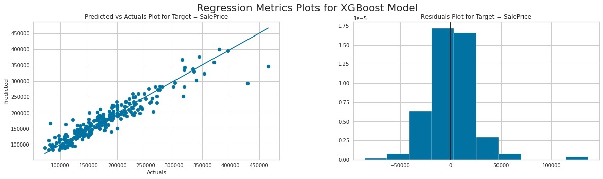
After fitting the training data, we can examine what has been done from the output. For example, we can see that AutoViML was doing preprocessing by filling the missing data. Similar to MLJAR, AutoViML also gives the visualized report. For the regression task, it visualizes the scatter plot of true and predicted values using the XGBoost model. It also plots the prediction residual error in a histogram. From the two plots, we can observe that the model has relatively good accuracy and the residual error is a normal distribution.
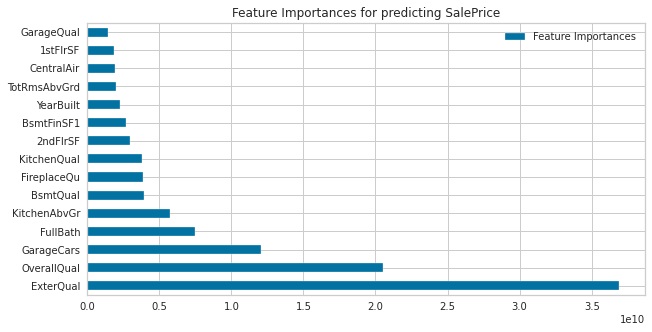
The next report is ensemble method trials. We can find this report for both regression and classification tasks. The last graph displays the feature importance. We can see that the most important feature to predict house prices is exterior material quality, followed by overall material and finish quality, and size of the garage respectively.
As for the classification task, it does not visualize the scatter plot, but the ROC curve for each of the four prediction classes, micro-average, and macro-average as well as the AUC value. We can see that all of the classes have AUC values above 0.98. The next chart reports the iso-f1 curves as the accuracy metric. It also later gives the classification report.
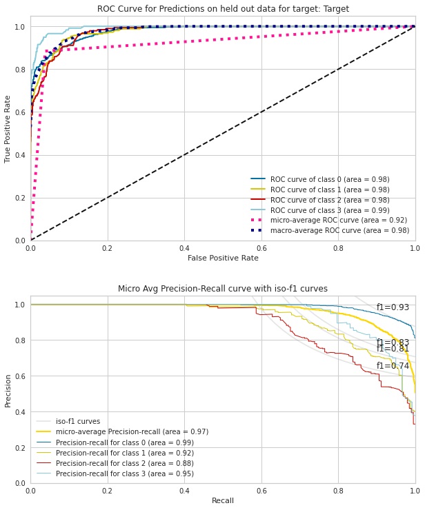
Average precision score, micro-averaged over all classes: 0.97
Macro F1 score, averaged over all classes: 0.83
#####################################################
              precision    recall  f1-score   support
           0       0.84      0.97      0.90       963
           1       0.51      0.59      0.54       258
           2       0.18      0.11      0.14       191
           3       0.00      0.00      0.00       118
    accuracy                           0.73      1530
   macro avg       0.38      0.42      0.40      1530
weighted avg       0.64      0.73      0.68      1530
[[938  19   6   0]
 [106 151   1   0]
 [ 53 117  21   0]
 [ 16  12  90   0]]
The following code prints out the result of AutoViML search. We can see that the best model is XGBRegressor and XGBClassifier for each task.
viml
Regression
XGBRegressor(base_score=0.5, booster='gbtree', colsample_bylevel=1,
             colsample_bynode=1, colsample_bytree=0.7, gamma=1, gpu_id=0,
             grow_policy='depthwise', importance_type='gain',
             interaction_constraints='', learning_rate=0.1, max_delta_step=0,
             max_depth=8, max_leaves=0, min_child_weight=1, missing=nan,
             monotone_constraints='()', n_estimators=100, n_jobs=-1, nthread=-1,
             num_parallel_tree=1, objective='reg:squarederror',
             predictor='cpu_predictor', random_state=1, reg_alpha=0.5,
             reg_lambda=0.5, scale_pos_weight=1, seed=1, subsample=0.7,
             tree_method='hist', ...)
Classification
CalibratedClassifierCV(base_estimator=OneVsRestClassifier(estimator=XGBClassifier(base_score=None,
                                                                                  booster='gbtree',
                                                                                  colsample_bylevel=None,
                                                                                  colsample_bynode=None,
                                                                                  colsample_bytree=None,
                                                                                  gamma=None,
                                                                                  gpu_id=None,
                                                                                  importance_type='gain',
                                                                                  interaction_constraints=None,
                                                                                  learning_rate=None,
                                                                                  max_delta_step=None,
                                                                                  max_depth=None,
                                                                                  min_child_weight=None,
                                                                                  missing=nan,
                                                                                  monotone_constraints=None,
                                                                                  n_estimators=200,
                                                                                  n_jobs=-1,
                                                                                  nthread=-1,
                                                                                  num_parallel_tree=None,
                                                                                  objective='binary:logistic',
                                                                                  random_state=99,
                                                                                  reg_alpha=None,
                                                                                  reg_lambda=None,
                                                                                  scale_pos_weight=None,
                                                                                  subsample=None,
                                                                                  tree_method=None,
                                                                                  use_label_encoder=True,
                                                                                  validate_parameters=None,
                                                                                  verbosity=None),
                                                          n_jobs=None),
                       cv=5, method='isotonic')
LightAutoML
Now, we have reached the 10th AutoML. LightAutoML is expected to be light as its name explains. Here, we set the task to be ‘reg’ for regression, ‘multiclass’ for multiclass classification, or ’binary’ for binary classification. We can also set the metrics and losses in the task. I set the timeout to be 3 minutes to let it find the best model. After simple .fit and .predict, we can already get the result.
Regression
!pip install -U https://github.com/sberbank-ai-lab/LightAutoML/raw/fix/logging/LightAutoML-0.2.16.2-py3-none-any.whl
!pip install openpyxl
from lightautoml.automl.presets.tabular_presets import TabularAutoML
from lightautoml.tasks import Task
# Create the model
light = TabularAutoML(task=Task('reg',), timeout=60*3, cpu_limit=4)
train_data = pd.concat([X_train, y_train], axis=1)
# Fit the training data
train_light = light.fit_predict(train_data, roles = {'target': 'SalePrice', 'drop':[]})
# Predict the validation data
pred_light = light.predict(X_val)
Classification
!pip install -U https://github.com/sberbank-ai-lab/LightAutoML/raw/fix/logging/LightAutoML-0.2.16.2-py3-none-any.whl
!pip install openpyxl
from lightautoml.automl.presets.tabular_presets import TabularAutoML
from lightautoml.tasks import Task
train_data = pd.concat([X_train, y_train], axis=1)
# Create the model
light = TabularAutoML(task=Task('multiclass',), timeout=60*3, cpu_limit=4)
# Fit the training data
train_light = light.fit_predict(train_data, roles = {'target': 'Target'})
# Predict the validation data
pred_light = light.predict(X_val)
The results for the classification task are the predicted class and the probability of each of the classes. In other words, the result fulfills multiclass and multilabel classification expectations.
# Convert the prediction result into dataframe
pred_light2 = pred_light.data
pred_light2 = pd.DataFrame(pred_light2, columns=['4','2','3','1'])
pred_light2 = pred_light2[['1','2','3','4']]
pred_light2['Pred'] = pred_light2.idxmax(axis=1)
pred_light2['Pred'] = pred_light2['Pred'].astype(int)
pred_light2.head()
| 1 | 2 | 3 | 4 | Pred | |
| 0 | 0.00 | 0.01 | 0.00 | 0.99 | 4 |
| 1 | 0.00 | 0.00 | 0.00 | 1.00 | 4 |
| 2 | 0.00 | 0.04 | 0.00 | 0.96 | 4 |
| 3 | 0.00 | 0.01 | 0.98 | 0.01 | 3 |
| 4 | 0.02 | 0.38 | 0.34 | 0.27 | 2 |
Conclusion
We have discussed 10 AutoML packages now. Please notice that there are still more AutoML not yet discussed in this post. Not only in Python notebook but AutoML also can be found in cloud computing or software. Which AutoML is your favourite? Or, do you have other AutoML in mind?

About Author
References
- Fig1 – https://www.kaggle.com/rendyk/automl-regression-part1
- Fig2- https://www.kaggle.com/rendyk/automl-regression-part1
- Fig3- Image by Author
- Fig4-Image by Author
- Fig5-Image by Author
- Fig6-Image by Author
- Fig7- https://www.kaggle.com/rendyk/automl-regression-part2
- Fig8- https://www.kaggle.com/rendyk/automl-regression-part2
- Fig9- https://www.kaggle.com/rendyk/automl-regression-part2
- Fig10- sklearn, topot, hyperopt, autokeras, mljar, autogluon, h2o, pycaret, autoviml
Connect with me here.


