A Comprehensive Guide on Databricks for Beginners
This article was published as a part of the Data Science Blogathon
Overview
Databricks in simple terms is a data warehousing, machine learning web-based platform developed by the creators of Spark. But Databricks is much more than that. It’s a one-stop product for all data needs, from data storage, analysis data and derives insights using SparkSQL, build predictive models using SparkML, it also provides active connections to visualization tools such as PowerBI, Tableau, Qlikview etc. It can be viewed as Facebook of big data.
Businesses generate a large amount of data, for example, Amazon has various operational data generation sources such as amazon app clicks, amazon pay, transaction data such as buying, re-order, cancellation, prime viewership data, it also has an amazon echo voice information, reviews and rating information, various sellers information across categories to name a few. The data engineering team handles various ETL to make sure the data is sourced, data is cleansed and quality checked and stored in data warehouses. In typical systems, without spark, a single task such as storing POS data to a SQL table can consume anywhere from 60 minutes to 600 minutes. But with Databricks all this is made easy using Spark. ETL’s are faster saving precious time and providing a competitive edge to stakeholders.
For example – Consider a loan approval batch pipeline that triggers every night at 9 PM with 100M applications, conventional models take days to evaluate the input data and provide an output, which leads to operational delays, and unhappy customers, case in point banking systems. What if the process is completed on the go, and the loan is approved in seconds as in fintech app’s, this is what Databricks brings to the table with an array of products and solutions. Faster ETL’s and easier decision making. Businesses take 24-48 hours to load weekly operations data to warehouses and this leads to delays in upcoming workflow and could lead to lost opportunities as well,
Databricks is integrated with Amazon Web Services, Microsoft Azure and Google Cloud Platform making it easy to integrate with these major cloud computing infrastructures. Some of the major firms such as Starbucks,
This article focuses on Databricks for data science enthusiasts. For more information check out the Databricks youtube page for the same.
Table of content
- Prior reading.
-
About Databricks community edition.
-
DataLake/Lakehouse.
-
Role-based Databricks adoption.
-
Advantages of Databricks.
-
Apache Spark
- Step by step guide –
-
Useful resources.
-
Data bricks certification.
-
Endnotes.
Prior Readings on Analytics Vidhya
Analytics Vidhya has quality content around pyspark, the goto language on Databricks, SQL and the Apache Spark framework. It would be immensely helpful to skim through them as well. Below are some relevant articles.
- PySpark for Beginners – Take your First Steps into Big Data Analytics (with Code)
- An Introduction to Data Analysis using Spark SQL
- Introduction to Spark MLlib for Big Data and Machine Learning
- How to use a Machine Learning Model to Make Predictions on Streaming Data using PySpark
- How to Connect DataBricks and MongoDB Atlas using Python API?
- Databricks and RStudio Launch Platform to make R Simpler than Ever for Big Data Projects!
About Databricks community edition
- Databricks community version is hosted on AWS and is free of cost.
- Ipython notebooks can be imported onto the platform and used as usual.
- 15GB clusters, a cluster manager and the notebook environment is provided and there is no time limit on usage.
- Supports SQL, scala, python, pyspark.
- Provides interactive notebook environment.
Databricks paid version has a 14 days trial period but needs to be used alongside AWS or Azure or GCP.
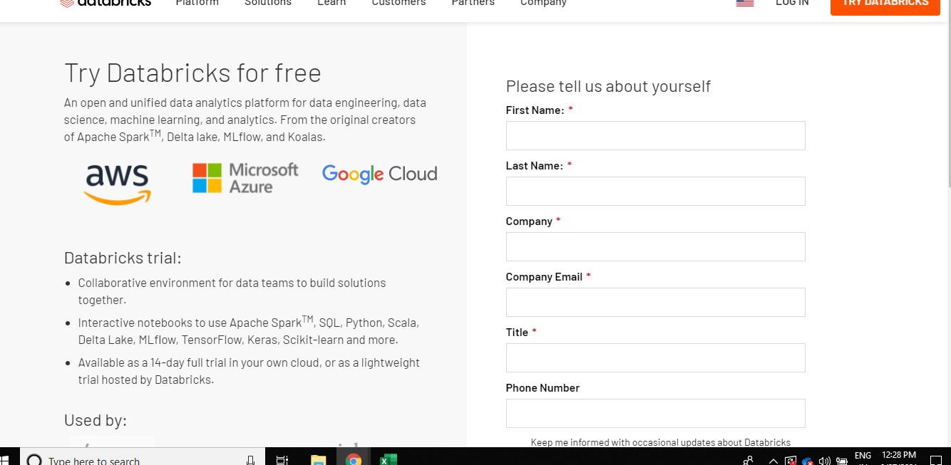
Image 2
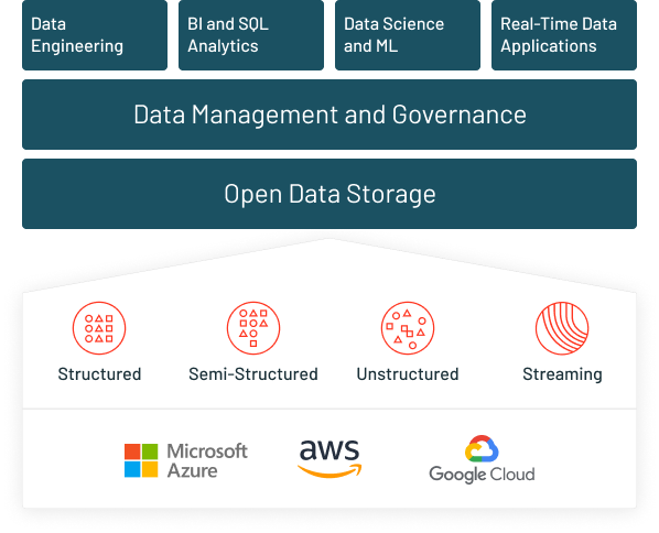
Data Lake
Lakehouse or data lake – is a marketing term used in Databricks for storage layer which can accommodate structured or unstructured, streaming or batch information. It’s a simple platform to store all data. Data lake from Databricks is called delta lake. Below are a few features of delta lake.
- It’s based on Parque file format.
- Compatible with Apache Spark.
- Versioning of data.
- ACID transactions – (atomicity, consistency, isolation, durability) ensure data durability and consistency.
- Batch and streaming data sink
- Supports deleting and upserting into tables using API’s
- Able to query millions of files using Spark
| Data Lake Grid |
Data lake
|
Data lakehouse |
Data warehouse
|
|
Types of data
|
All types: Structured data, semi-structured data, unstructured (raw) data | All types: Structured data, semi-structured data, unstructured (raw) data | Structured data only |
| Cost | $ | $ | $$$ |
| Format | Open format | Open format | The closed, proprietary format |
| Scalability | Scales to hold any amount of data at low cost, regardless of the type | Scales to hold any amount of data at low cost, regardless of the type | Scaling up becomes exponentially more expensive due to vendor costs |
|
Intended users
|
Limited: Data scientists | Unified: Data analysts, data scientists, machine learning engineers | Limited: Data analysts |
|
Ease of use
|
Difficult: Exploring large amounts of raw data can be difficult without tools to organize and catalog the data | Simple: Provides simplicity and structure of a data warehouse with the broader use cases of a data lake | Simple: The structure of a data warehouse enables users to quickly and easily access data for reporting and analytics |
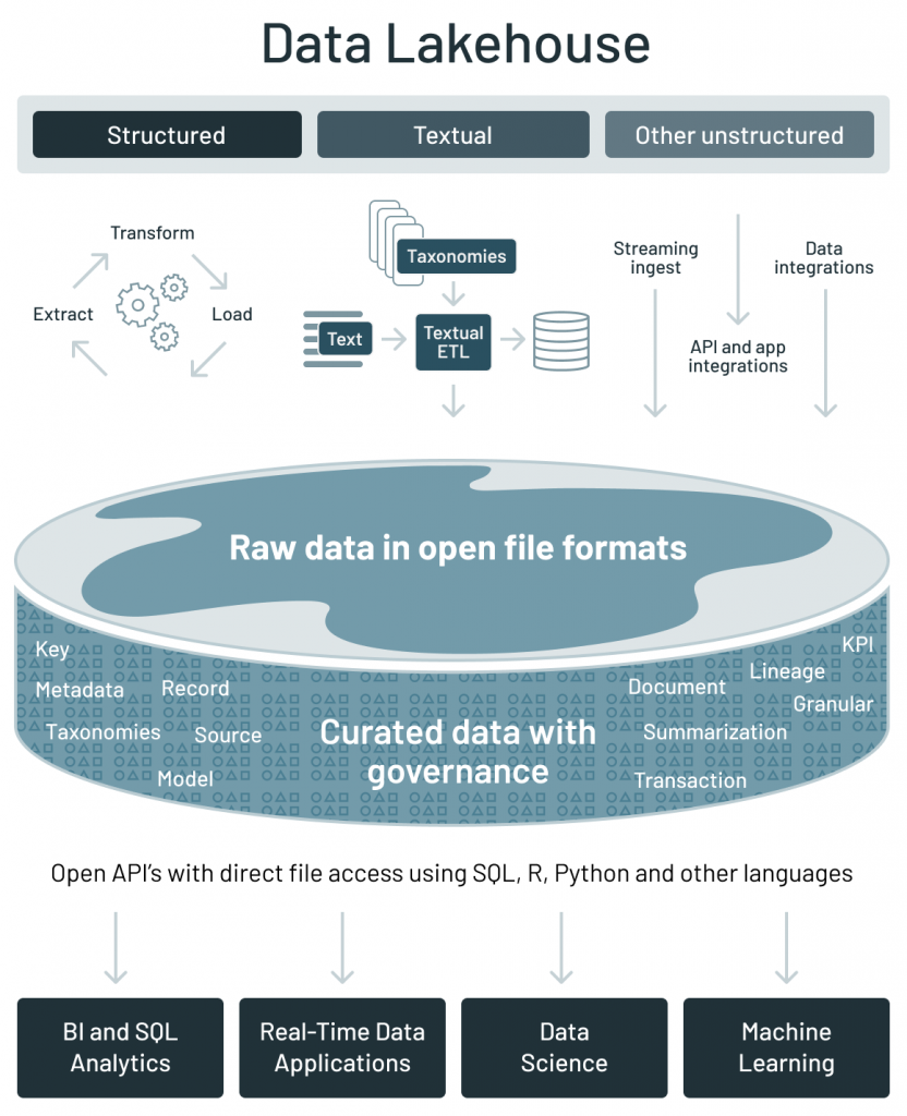
Image 3
Role-based Databricks adoption
Data Analyst/Business analyst: As analysis, RAC’s, visualizations are the bread and butter of analysts, so the focus needs to be on BI integration and Databricks SQL. Read about Tableau visualization tool here.
Data Scientist: Data scientist have well-defined roles in larger organizations but in smaller organizations, data scientist wears various hats, one can own all the 3 roles, of an analyst, data engineer, bi visualizer etc. In a well-defined role, data scientists are responsible to source data, a skill grossly neglected in the face of modern ML algorithms. Build predictive models, manage model deployment. Monitor data drift,
Important skills
- Sourcing data – Identify data sources, and leverage them to build holistic models.
- Build predictive models.
- Model lifecycle.
- Model deployment.
Data Engineer: Largely responsible to build ETL’s, and manage the constant flow of ever-increasing data. Process, clean, and quality check the data before pushing it to operational tables. Model deployment and platform support are other responsibilities entrusted to data engineers.
Databricks have to be combined either with Azure/AWS/GCP and due to its relatively higher costs, adoption of it in small/medium startups is quite low in India.
Advantages of Databricks
- Support for the frameworks (scikit-learn, TensorFlow,Keras), libraries (matplotlib, pandas, numpy), scripting languages (e.g.R, Python, Scala, or SQL), tools, and IDEs (JupyterLab, RStudio).
-
Databricks delivers a Unified Data Analytics Platform, data engineers, data scientists, data analysts, business analysts can all work in tandem on the same notebook.
-
Flexibility across different ecosystems – AWS, GCP, Azure.
-
Data reliability and scalability through delta lake.
-
Basic built-in visualizations.
-
AutoML and model lifecycle management through MLFLOW.
-
Hyperparameter tuning support through HYPEROPT.
-
Github and bitbucket integration
- 10X Faster ETL’s.
Apache Spark
Spark is a tool to coordinate tasks/jobs across a cluster of computers. These clusters of machines are managed by a cluster manager, it could be either YARN(yet another resource negotiator) or Mesos or Sparks own Standalone cluster manager. It supports languages such as Scala, Python, SQL, Java, and R. Spark application consists of one driver and executors.
The driver node is responsible for three things:
- Maintaining information about the Spark application;
- Responding to a user’s program.
- Analyzing, distributing, and scheduling work across the executors.
The executors are responsible for two things:
- Executing code assigned to it by the driver.
- Reporting the state of the computation, on that executor, back to the driver node.
The cluster manager is responsible:
- Controlling physical machines and allocates resources to Spark applications.
Check out this article for an indepth understanding of Spark – Understand The Internal Working of Apache Spark.
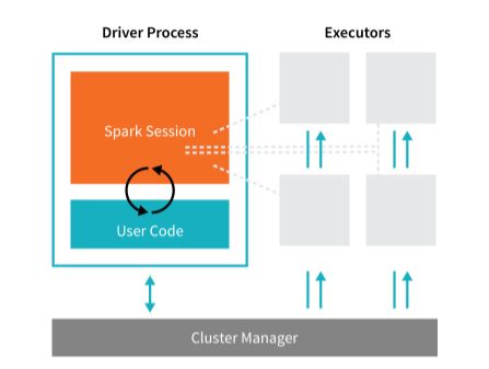
Image 4
Step by step guide to Databricks
Databricks community edition is free to use, and it has 2 main Roles 1. Data Science and Engineering and 2. Machine learning. The machine learning path has an added model registry and experiment registry, where experiments can be tracked, using MLFLOW. Databricks provides Jupyter notebooks to work on, which can be shared across teams, which makes it easy to collaborate.
Create a cluster:
For the notebooks to work, it has to be deployed on a cluster. Databricks provides 1 Driver:15.3 GB Memory, 2 Cores, 1 DBU for free.
- Select Create, then click on cluster.
- Provide a cluster name.
- Select Databricks Runtime Version – 9.1 (Scala 2.12, Spark 3.1.2) or other runtimes, GPU aren’t available for the free version.
- Select the availability zone as AUTO, it will configure the nearest zone available.
- It might take a few minutes before the cluster is up and running.
-
The cluster will automatically terminate after an idle period of two hours.
- To close the cluster there are 2 options, one is to terminate and then restart later. Secondly, delete the cluster entirely. Deleting the cluster will not delete the notebook as notebooks can be mounted on any available cluster relevant to the job at hand.
Alternatively
- Select Compute
- Select on create cluster and then follow step 2 onwards given above.
Create a notebook:
- Select create option and then click on notebook.
- Provide a relevant name to the notebook.
- Select language of preference – SQL, Scale, Python, R.
- Select a cluster for the notebook to run on.
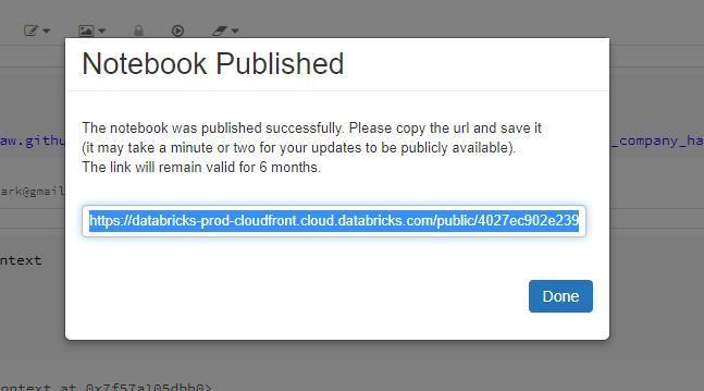
Publish workbook:
Once the analysis is complete, Databricks notebooks can be published(publicly available) and the links will be available for 6 months.
Import published notebook:
Databricks notebooks, which are published can be imported using URL as well as physical files. To import using URL.
- Select Workspace and move to the folder to which the file needs to be saved.
- Click on import and then a new dialog box appears.
- Paste the URL to and click on import.
- Use the link and import a sparkSQL tutorial to the workspace.
Run SQL on Databricks
Create a new notebook and select SQL as the language. In the notebook, select the Upload Data and upload the csv.
Write the data to events002
%python
df1 = spark.read.format("csv").load("dbfs:/FileStore/shared_uploads/[email protected]/test-3.csv",header="true", inferSchema="true")
df1.write.format("delta").mode("overwrite").save("/mnt/delta/events002")
Create a SQL table using the below code:
DROP TABLE IF EXISTS diamonds;
CREATE TABLE diamonds USING DELTA LOCATION '/mnt/delta/events002/'
Run SQL commands to query data:
select * from diamonds limit 10
select manufacturer, count(*) as freq from diamonds group by 1 order by 2 desc
Visualize the SQL output on Databricks notebook
The output data-frames can be visualized directly in the notebook. Select the bar icon below and choose the appropriate chart. A total of 11 chart types are available.
- Bar chart
- Scatter chart
- Maps
- Line chart
- Area chart
- Pie chart
- Quantile chart
- Histogram
- Box plot
- Q-Q plot
- Pivot (Excel-like pivot chart interface. )
End to end machine learning classification on Databricks
Databricks machine learning support is growing day by day, MLlib is Spark’s machine learning (ML) library developed for machine learning activities on Spark. Below is a classification example to predict the quality of Portuguese “Vinho Verde” wine based on the wine’s physicochemical properties.
Download the data using the link, download both winequality-red.csv and winequality-white.csv to your local machine. And upload the CSV using the Upload Data command in the toolbar.
import pandas as pd

red_wine = pd.read_csv("/dbfs/FileStore/shared_uploads/[email protected]/winequality_red.csv")
white_wine = pd.read_csv("/dbfs/FileStore/shared_uploads/[email protected]/winequality_white.csv")
white_wine['is_red'] = 0.0
red_wine['is_red'] = 1.0
data_df = pd.concat([white_wine, red_wine], axis=0)
Plotting :
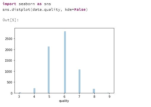
Plot a histogram of the Y label:
import seaborn as sns
sns.distplot(data.quality, kde=False)
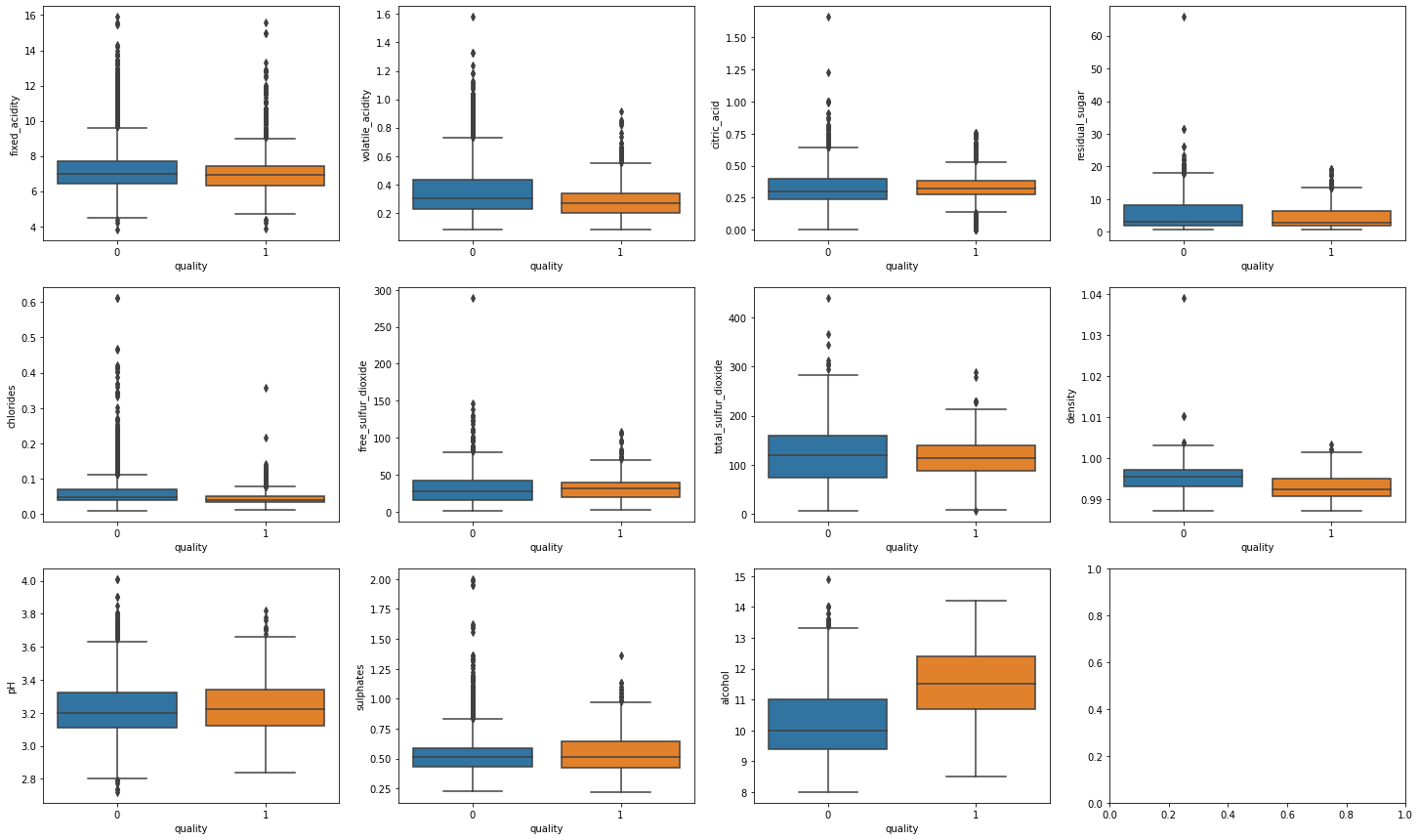
Box plots to compare features and Y label:
import matplotlib.pyplot as plt
dims = (3, 4)
f, axes = plt.subplots(dims[0], dims[1], figsize=(25, 15))
axis_i, axis_j = 0, 0
for col in data.columns:
  if col == 'is_red' or col == 'quality':
    continue # Box plots cannot be used on indicator variables
  sns.boxplot(x=high_quality, y=data[col], ax=axes[axis_i, axis_j])
  axis_j += 1
  if axis_j == dims[1]:
    axis_i += 1
    axis_j = 0
Split train test data:
from sklearn.model_selection import train_test_split
train, test = train_test_split(data, random_state=123)
X_train = train.drop(["quality"], axis=1)
X_test = test.drop(["quality"], axis=1)
y_train = train.quality
y_test = test.quality
Build a baseline Model:
import mlflow
import mlflow.pyfunc
import mlflow.sklearn
import numpy as np
import sklearn
from sklearn.ensemble import RandomForestClassifier
from sklearn.metrics import roc_auc_score
from mlflow.models.signature import infer_signature
from mlflow.utils.environment import _mlflow_conda_env
import cloudpickle
import time
# The predict method of sklearn's RandomForestClassifier returns a binary classification (0 or 1).
# The following code creates a wrapper function, SklearnModelWrapper, that uses
# the predict_proba method to return the probability that the observation belongs to each class.
class SklearnModelWrapper(mlflow.pyfunc.PythonModel):
  def __init__(self, model):
    self.model = model
  def predict(self, context, model_input):
    return self.model.predict_proba(model_input)[:,1]
# mlflow.start_run creates a new MLflow run to track the performance of this model.
# Within the context, you call mlflow.log_param to keep track of the parameters used, and
# mlflow.log_metric to record metrics like accuracy.
with mlflow.start_run(run_name='untuned_random_forest'):
  n_estimators = 10
  model = RandomForestClassifier(n_estimators=n_estimators, random_state=np.random.RandomState(123))
  model.fit(X_train, y_train)
  # predict_proba returns [prob_negative, prob_positive], so slice the output with [:, 1]
  predictions_test = model.predict_proba(X_test)[:,1]
  auc_score = roc_auc_score(y_test, predictions_test)
  mlflow.log_param('n_estimators', n_estimators)
  # Use the area under the ROC curve as a metric.
  mlflow.log_metric('auc', auc_score)
  wrappedModel = SklearnModelWrapper(model)
  # Log the model with a signature that defines the schema of the model's inputs and outputs.
  # When the model is deployed, this signature will be used to validate inputs.
  signature = infer_signature(X_train, wrappedModel.predict(None, X_train))
  # MLflow contains utilities to create a conda environment used to serve models.
  # The necessary dependencies are added to a conda.yaml file which is logged along with the model.
  conda_env =  _mlflow_conda_env(
        additional_conda_deps=None,
        additional_pip_deps=["cloudpickle=={}".format(cloudpickle.__version__), "scikit-learn=={}".format(sklearn.__version__)],
        additional_conda_channels=None,
    )
  mlflow.pyfunc.log_model("random_forest_model", python_model=wrappedModel, conda_env=conda_env, signature=signature)
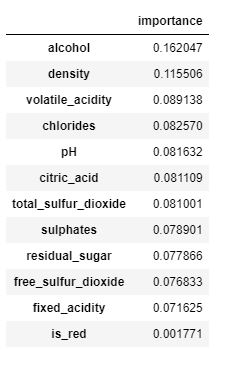
Derive feature importance:
feature_importances = pd.DataFrame(model.feature_importances_, index=X_train.columns.tolist(), columns=['importance'])
feature_importances.sort_values('importance', ascending=False)
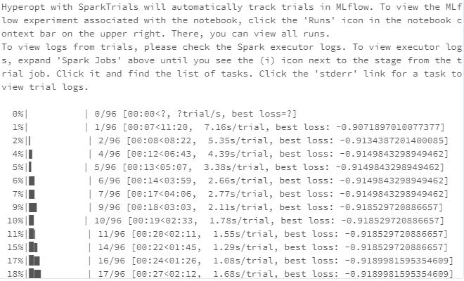
Experiment with XGBoost and Hyperopt:
Hyperopt is a hyperparameter tuning framework based on bayesian optimization. Grid search is time-consuming and Random search while better than grid search, fails to provide optimum results. Hyperopt know-how article on Analytics Vidhya.
from hyperopt import fmin, tpe, hp, SparkTrials, Trials, STATUS_OK
from hyperopt.pyll import scope
from math import exp
import mlflow.xgboost
import numpy as np
import xgboost as xgb
search_space = {
  'max_depth': scope.int(hp.quniform('max_depth', 4, 100, 1)),
  'learning_rate': hp.loguniform('learning_rate', -3, 0),
  'reg_alpha': hp.loguniform('reg_alpha', -5, -1),
  'reg_lambda': hp.loguniform('reg_lambda', -6, -1),
  'min_child_weight': hp.loguniform('min_child_weight', -1, 3),
  'objective': 'binary:logistic',
  'seed': 123, # Set a seed for deterministic training
}
def train_model(params):
  # With MLflow autologging, hyperparameters and the trained model are automatically logged to MLflow.
  mlflow.xgboost.autolog()
  with mlflow.start_run(nested=True):
    train = xgb.DMatrix(data=X_train, label=y_train)
    test = xgb.DMatrix(data=X_test, label=y_test)
    # Pass in the test set so xgb can track an evaluation metric. XGBoost terminates training when the evaluation metric
    # is no longer improving.
    booster = xgb.train(params=params, dtrain=train, num_boost_round=1000,
                        evals=[(test, "test")], early_stopping_rounds=50)
    predictions_test = booster.predict(test)
    auc_score = roc_auc_score(y_test, predictions_test)
    mlflow.log_metric('auc', auc_score)
    signature = infer_signature(X_train, booster.predict(train))
    mlflow.xgboost.log_model(booster, "model", signature=signature)
    # Set the loss to -1*auc_score so fmin maximizes the auc_score
    return {'status': STATUS_OK, 'loss': -1*auc_score, 'booster': booster.attributes()}
# Greater parallelism will lead to speedups, but a less optimal hyperparameter sweep.
# A reasonable value for parallelism is the square root of max_evals.
spark_trials = SparkTrials(parallelism=10)
# Run fmin within an MLflow run context so that each hyperparameter configuration is logged as a child run of a parent
# run called "xgboost_models" .
with mlflow.start_run(run_name='xgboost_models'):
  best_params = fmin(
    fn=train_model,
    space=search_space,
    algo=tpe.suggest,
    max_evals=96,
    trials=spark_trials,
    rstate=np.random.RandomState(123)
  )
Finally, retrieve the best model from MLFLOW run :
best_run = mlflow.search_runs(order_by=['metrics.auc DESC']).iloc[0]
print(f'AUC of Best Run: {best_run["metrics.auc"]}')
Practice – Market Basket Analysis on Databricks
Use the online notebook to analyse InstaKart grocery data and recommended upselling/cross-selling opportunities using market basket analysis.
Dashboarding on Databricks:
Databricks has a feature to create an interactive dashboard using the already existing codes, images and output.
- Move to View menu and select + New Dashboard
- Provide a name to the dashboard.
- On the Top Right corner of each cell click on the tiny Bar Graph image.
- It will show the available dashboard for the notebook.
- If the code block or image needs to be on the dashboard, tick the box.
- All ticked cells will appear on the dashboard.
- The cell and be organised as necessary easily with the drag and drop feature.
Useful resources and references
- Forecasting at Starbucks using Databricks.
- Databricks community for discussion on various topics.
- Databricks university alliance – Provides university teachers as well as students complimentary access to the platform.
- Webinars and Ebooks from Databricks.
- Ebook on delta lake.
- Ebook on ML lifecycle.
- Datalake Databricks explanation
- Dashboarding on Databricks.
Databricks Certification
Databricks provides live instructor lead training, as well as self-paced programs to help individuals understand the platform better. The self-paced course is priced at $2000. It also provides certification based on role fitment. The common career tracks are Business leader, platform admin, SQL analyst, data engineer, data scientist.
There are four certifications, namely
- Databricks certified associate developer for Apache Spark – For spark developers.
- Databricks Certified Professional Data Scientist – For all things ML.
- Azure Databricks Certified Associate Platform Administrator – is an exam to assesses the understanding of basics in network infrastructure and security, identity and access, cluster usage, and automation with the Azure Databricks platform.
- Databricks Certified Professional Data Engineer – All things ETL, pipelines, and deployment.
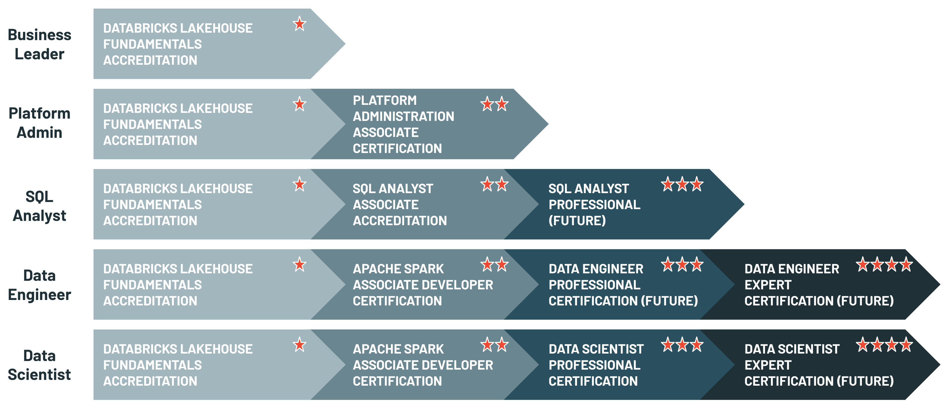
Image 5
End Notes
This article just scratches the surface of what Databricks is capable of. Databricks is capable of a lot more, which are not explored in this article, and for data enthusiasts, it is quite a treasure throve. So practice and always keep learning.
Good luck! Here is my Linkedin profile in case you want to connect with me. I’ll be happy to be connected with you. Check out my other articles on data science and analytics here.
Image References :
Image 1: https://databricks.com/product/data-lakehouse
Image 2: https://databricks.com/try-databricks
Image 3: https://databricks.com/blog/2021/05/19/evolution-to-the-data-lakehouse.html
Image 4: https://pages.databricks.com/definitive-guide-spark.html
Image 5: jsdsdhttps://academy.databricks.com/catalog
Data scientist! Extensively using data mining, data processing algorithms, visualization, statistics and predictive modelling to solve challenging business problems and generate insights.


