Numpy Refresher for Beginners (with Anaconda Setup)

This article was published as a part of the Data Science Blogathon

Introduction

“Machine Learning can change the future”, this line you might have heard thousands of times if you belong to the technology, indeed it can, we all know the answer, but how will it? You might have heard or seen Autonomous Vehicles, Smart Chips for the brain, Image Regeneration, etc. but what if you want to try out all these things, you would have to start from somewhere right? don’t worry I got you, you are at the right place as starting from this article I would be writing a series of Deep Learning Articles that would help you get started in the Deep Learning Industry.

These articles would be purely based on Python language and its libraries. I would be giving both theoretical and practical examples wherever needed. So stay tuned and I would suggest reading it at your pace.

Every war that has been fought needs weapons and tools similarly if you want to enter any field you need to have some set of tools that would help you go ahead in the field. Here the tool is Anaconda (don’t worry it’s not the snake).

This article is divided into two sections. The first section is about setting up the Anaconda Environment Where we would be discussing the following:

1. what is Anaconda?
2. Anaconda Installation
3. What are Python Packages?
4. Managing python packages
5. Managing Environments

While the second one would be a refresher for your matrix concepts that are the soul of Neural Network calculations. In this section we would be discussing the following:

1. Data Dimensions
2. Numpy Data
3. Elementwise data operations
4. Matrix Multiplication
5. Matrix Transpose

So let’s start with understanding the tools that are required to set foot in Deep Learning.

Anaconda Setup

In this section let’s set up the Anaconda Environment.

What is Anaconda?

Anaconda is a program that helps in managing python packages, environments, editors, and notebooks for python language. It’s a UI-based program where users can simply search for packages and editors and create environments to work on.

If you already have the python language installed in your system it’s no problem you can still install Anaconda and use it or else you can just install Anaconda which would come up with the required python version. Anaconda already comes up with a bunch of python packages, a package management system (PIP), and environmental management system (Conda) which makes it easy to use.

The typical size of this program is around 500MB since it already comes up with some python packages, and comes up with the following things:

1. Python: A specific version of python language based on anaconda’s version.

2. Conda: A command-line utility for environments and packages management that works the same way in both Unix and Windows environments.

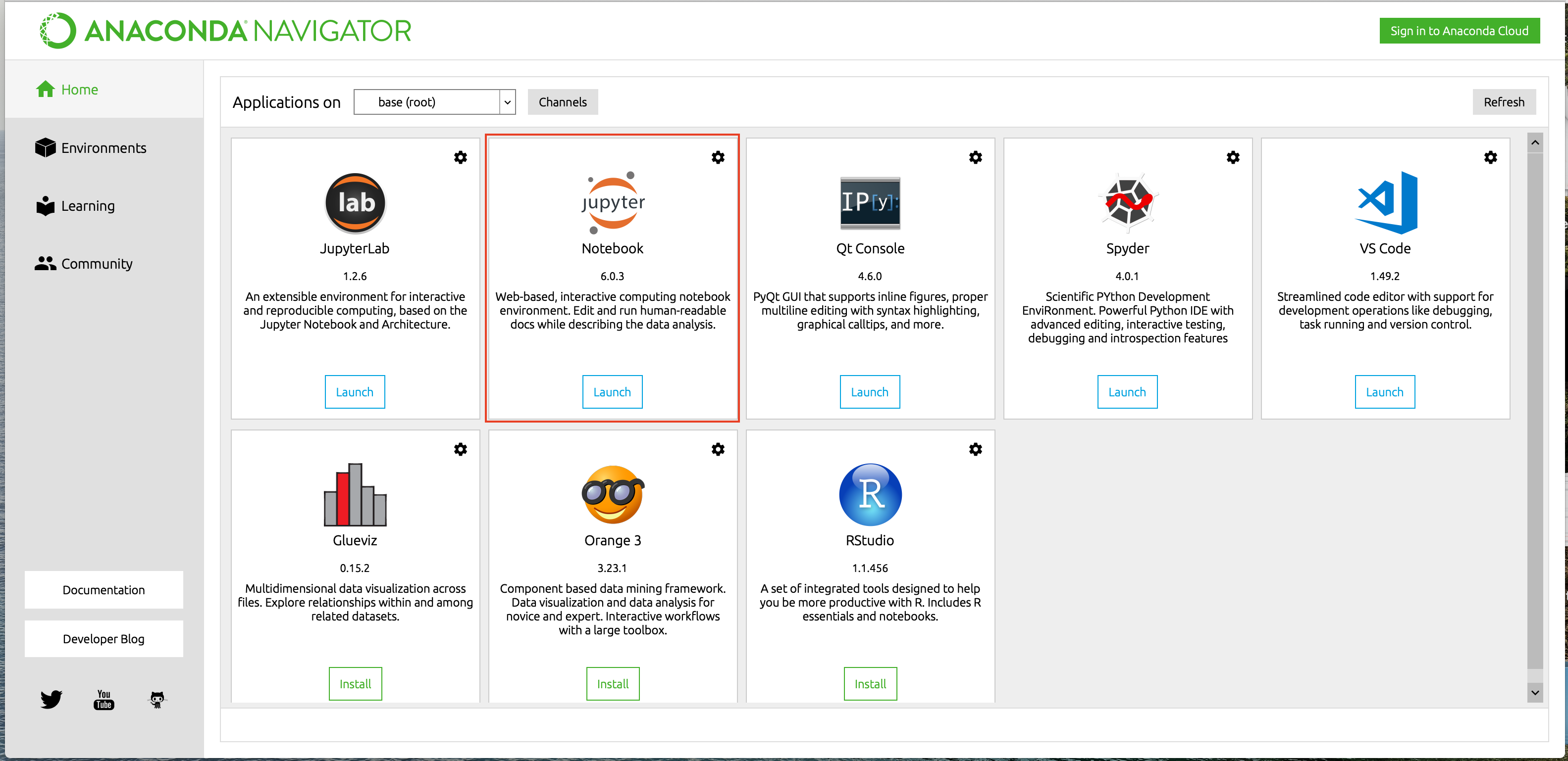
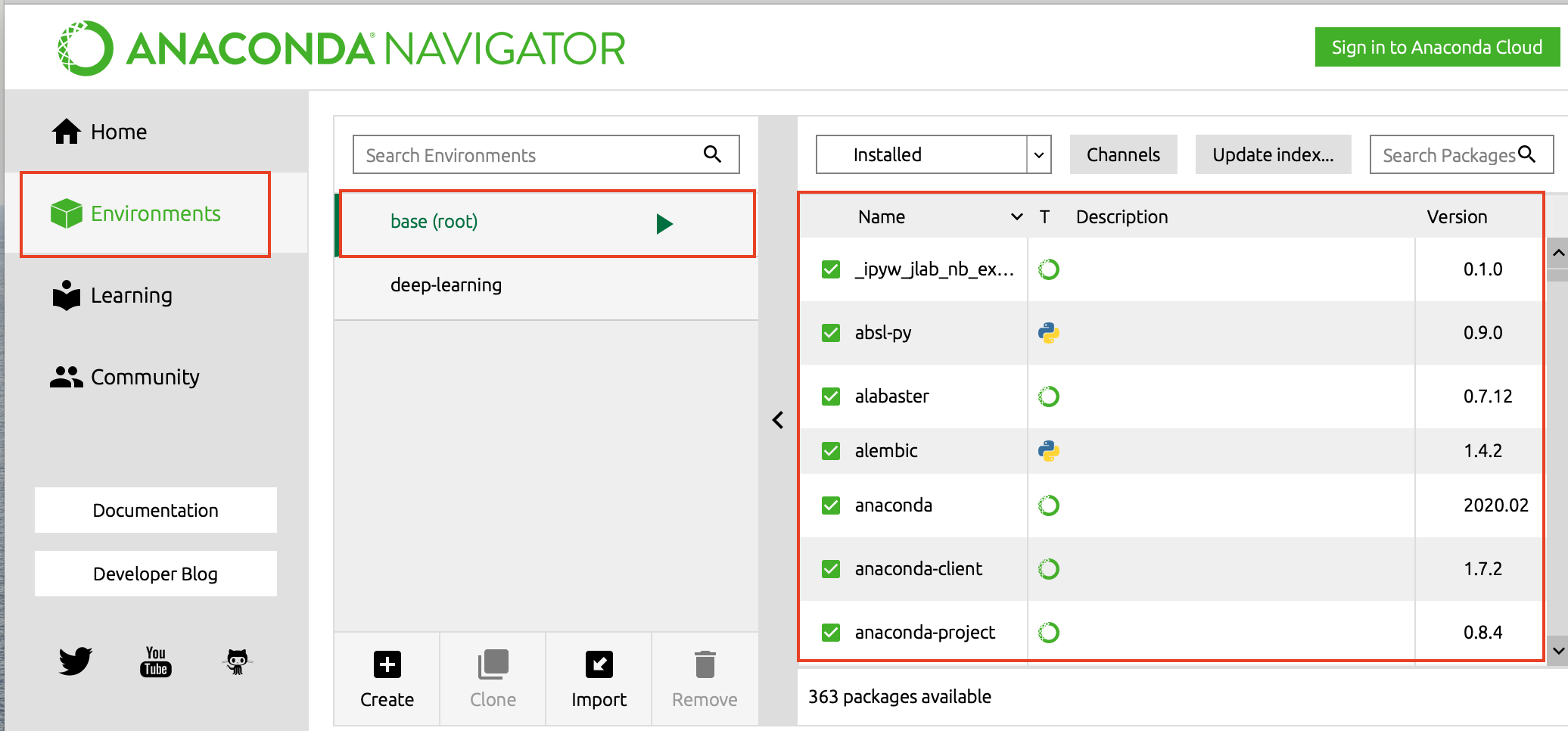
3. Anaconda Navigator: it’s a UI with which users can interact, check and install the packages and start multiple python related applications.

Anaconda Installation

Anaconda is available for both Windows and Unix environments, which you can download from the following link https://www.anaconda.com/products/individual. Once you have downloaded the tool you can open it and the following window would prompt up:

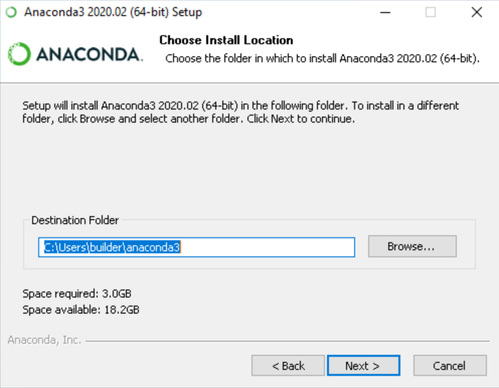
You can choose the path where you want to install the anaconda, I will suggest let it be the default location only. once done click on the Next button which will lead you to the following.

 

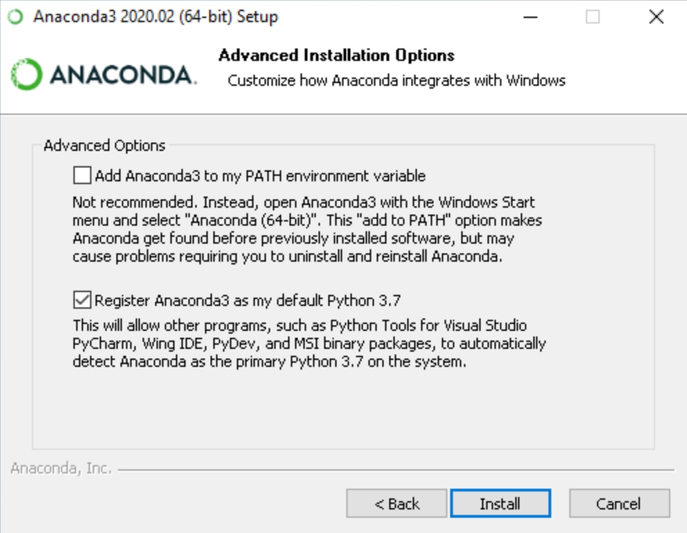
If you have python already installed then you can go ahead with the mentioned settings otherwise you can add Anaconda3 to your python path by selecting the first option. Once done click on install button to go ahead and install the anaconda in your system. The final window would look something like this once the installation is done.

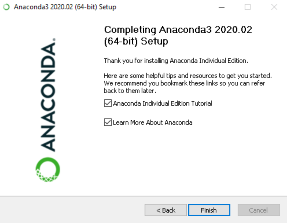
You can verify the installations by starting “Anaconda Prompt” in your system. As Anaconda is now installed let’s jump to understanding the python packages.

What is a Python package?

A Python package is a collection of modules/functions where each module is designed to solve a specific task. You can simply import the modules using the word “import” and specifying the module or submodule name eg. import numpy (Numpy is a module used for scientific computations).

If you want to create your own package you can create a Python file with some modules implemented using OOPS and publish it on pypi.org and then everyone would be able to access it. 

Anaconda already comes up with a bunch of Python packages that may be useful for you if not you can delete them if needed. 

Managing Python Packages:

Python package management can be done using two utilities PIP or Conda. These are called Python Package Managers that can help in the installation, deletion, and management of the Python packages. The only difference between these two is Conda manages the packages that are available from Anaconda distribution while PIP is the default package management system for Python. You can download your required package just by specifying the following command:

$ pip install package_name
$ conda install package_name

Which one should you prefer PIP or Conda?

Packages that are specific to Data Science and Machine Learning are preferably installed using Conda, while PIP can be used for general package installations.

For deleting any package you can delete it using PIP only even if it was downloaded from Conda:

$ pip uninstall package_name

Managing Environments:

A Python environment is the collection of the following entities:

Anaconda comes up with a base environment that has all the preinstalled packages. You can have an environment inside that base environment or you can create a whole new one. These environments are called “Virtual Environments”.

Why do we need multiple environments?

If we want to create multiple Machine Learning based algorithms which use different package versions you can not have the same package with multiple versions in the same environment so you need to have multiple environments, so the basic purpose of having multiple environments is to keep the development isolated.

This often happens when you work on projects that have Python2 and Python3 based dependencies since both of these versions have different sets of libraries compatibility.

How to create a virtual environment?

To create a virtual environment you need to install the python package named “virtualenv”.  You can download it using the following command:

$ pip install virtualenv

Once the library is installed you can create the environment using the following command:

$ virtualenv my_env

this command would create a virtualenv with the name “my_env”,  and to activate this you can use the following command:

Windows:

$ my_envScriptsactivate

Unix:

$ source my_env/bin/activate

This would activate the environment now you can go ahead and install the required packages in the environment.

Numpy Refresher

Now that you know how to set up Anaconda it’s time for you to have a refresher about the matrix and various matrix manipulation techniques. Deep learning calculations are built on top of matrix math so you need to have a thorough knowledge of it to start building your own Neural Networks. One of the beauties of Python language is that it comes up with the ability to process these matrices through a library named Numpy.

Data Dimensions using Numpy

Neural Networks do a lot of maths in the backend to predict a value or to classify the data. One important thing we must know is how that data is represented ? or What is the shape of the data? For example, a number can represent a single entity while a list of numbers can tell a lot of other information, or for instance, an image has a set of pixel values that are also represented in some order.

Data that we use for NN calculations are classified into three different categories based on their dimension. These categories are as follows:

1. Scalar Values: This is just a single numerical value like 1, 3, 7.6, etc. Scaler values have no dimensions at all or are often called zero-dimensional data.

2. Vectors: These are a list of scalar values that are typical of two types, Row Vector and Column Vector. The basic difference between these two is they store data in a horizontal and vertical manner respectively.

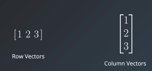
Vectors have only one dimension and are of various lengths depending on the number of elements they have.

3. Matrics: These are the collection of values arranged in rows and columns order. Matrices are two-dimensional data types represented using mxn, where m is the number of rows and n is the number of columns.

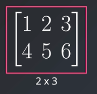
In the above image, you can clearly see the matrix of dimension 2×3 that has 2 rows and 3 columns.

4. Tensors: These are n-dimensional values, just to be specific anything above a two-dimensional matrix is called a tensor. Normally these are hard to visualize so we consider them as the collection of vectors depending on their dimensions.

Numpy data

Each and every data dimension that we have seen can be represented in python using numerical values or lists, but the only issue is Python can be a bit slow while doing data manipulation. normally we see tensors of dimension 10×20 or 5×10 but in real-world data, dimensions can be much higher so doing computations would be even slower. So is there any way we can fasten these manipulations? Yes, Python provides one such library called NumPy whose computation speed is must faster than list comprehension. Now let’s start exploring Numpy for a bit.

Numpy Installation

NumPy is available on PyPI so you can directly install it using PIP.

$ pip install numpy

Importing Numpy

To import NumPy in your code you can write the following code:

import numpy as np

The most common Numpy objects are ndarray, which are similar to python lists but can have n number of dimensions and are faster than list manipulation. Now let’s discuss each data dimension in NumPy.

Scalars:

NumPy scalers are a bit different than Python scalar values, they allow users to specify signed and unsigned types along with their data types like uint8, uint16, etc. There is no specific function in NumPy to define a scalar so we have to use the array function only while providing the scalar value.

s = np.array(5)

To check the shape of the above scalar you can write the following code:

s.shape

this gives the output (), indicating it has zero dimensions.

Vectors:

Creating vectors in NumPy is easy, you just need to pass the list for which you need to create the vector.

v = np.array([1,2,3])
v.shape

The shape of the above vector is (3,) as it has 3 rows and dimensionality of 1. You can access various elements of this vector by just passing their index like this:

v[0]

this would return element “1” as default indexing for NumPy starts with 0. To get a series of elements starting from an index you can write the following:

v[1:]

This would return all the elements starting from index 1. To get the list of elements to a particular index you can use the following:

v[:2]

This would return all the elements starting from index 0 to 1 as arrays have defaulted from 0 and the upper bound of the array would always be “upper bound – 1” i.e. 2-1 = 1, and finally if you want to slice the vector you can use the following:

v[0:2]

This would return elements from index 0 to 1 as the last number is not included in the bound.

Matrices:

Matrices are multi-dimensional lists, so NumPy uses these multidimensional lists to obtain the NumPy matrices.

m = np.array([[1,2,3], [4,5,6], [7,8,9]])
m.shape

Here we have created a matrix of shape (3,3) i.e. three rows and three columns respectively. To access the index-wise elements we need to define the row and column number of the element (again indexing for both rows and columns starts from 0).

m[1][2]

This returns the element belonging to row 1 and column 2 i.e. 2. and for Slicing the matrix you can again use “:” for both rows and columns.

Tensors: 

It’s the matrix with a higher number of dimensions. and can be defined as follows:

t = np.array([[[[1],[2]],[[3],[4]],[[5],[6]]],[[[7],[8]],
[[9],[10]],[[11],[12]]],[[[13],[14]],[[15],[16]],[[17],[17]]]])

t.shape

The shape of the given tensor is (3, 3, 2, 1), and you can access each and every element of the tensor in the same fashion as matrix eg. t[1][1][1][0].

Element wise Data Operations using NumPy

Applying mathematics operations on scaler values is easy right? but when it comes to lists, vectors, matrices, and tensors we need to apply the same operation for each number of elements. Here scalers are defined as one category while all other forms of data are considered the same as they all have a list of data.

Scaler and Matrix operation:

To perform mathematical operations between scaler value and the matrix we just need to write them together and perform the operation to each element of the matrix, for example:

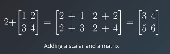
As you can see in the above image scaler value 2 is added to each and every element of the matrix resulting in a new matrix. All other mathematical operations like subtraction, division, and multiplication can be applied between scaler and matrix values in the same way.

Now let’s check the code part for scaler and matrix operations. The traditional way of doing it is to iterate over each value in the matrix and do the mathematical operation with the given scaler value.

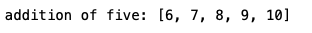
values = [1,2,3,4,5]
for i in range(len(values)):
    values[i] += 5
print('addition of five:', values)

 

The only issue here is it increases the time complexity as we are iterating over each element and performing the operation. The only solution to this is using NumPy which can accelerate the computation. To do the same operation in the NumPy way you would have to do the following:

import numpy as np

values = [1,2,3,4,5]

values = np.array(values) + 5

print('addition of five using numpy:', values)

Here you can see that just converting the list to NumPy array and then adding scaler value to the vector is very similar to adding two scaler values. Other mathematical operations are applied in the same way for scaler to matrix operation.

Matrix and Matrix operation in NumPy

For a matrix to matrix operation, all the matrices should have the same shape to perform the mathematical operation, for example:

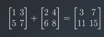
As you see both the matrix are of the same shape (2×2) and addition operations are performed for each respective element. a[0] [0] is added to the b[0][0] and so on. Other mathematical operations like subtraction and division can be applied in the same fashion as the addition, only the multiplication operation is different from all these operations.

For matrix to matrix operation again you can go ahead with iterating over each value in the matrices and perform the mathematical operations but that is again time-consuming so you would be using the same NumPy solution.

import numpy as np 
a = np.array([[1,3],[5,7]])
print('a =', a, 'n')
b = np.array([[2,4],[6,8]])
print('b =', b, 'n')
print('a+b = ', a + b)

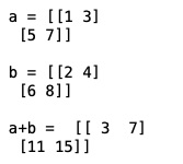
Here you can see both the matrix are of the same shape and produced the desired output as applied operation. Similarly, subtraction and division operations can be formed in the same way.

Let’s check what happens when you apply any operation between matrices of two different shapes.

import numpy as np 
a = np.array([[1,3],[5,7]])
print('a =', a, 'n')
c = np.array([[2,3,6],[4,5,9],[1,8,7]])
print('c =', c, 'n')
print('a+c = ', a + c)

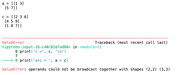
 You can see in the given image that the code has thrown an error that both the matrices are of different shapes.

Matrix Multiplication in NumPy

When we talk about matrix multiplication the operation is the same as any other operation.

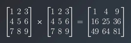
As you can see in the image that elements from one matrix are being multiplied by the respective element in the other matrix.

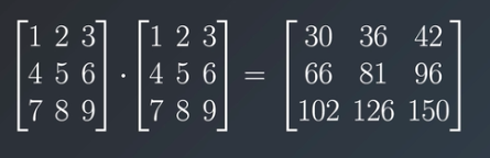
But usually, in Neural Networks math matrix multiplication is the term used for matrix dot product which is a lot different from matrix multiplication. The major difference here is that the matrices shape should be mxn and nxp respectively i.e first matrix’s number of columns should be equal to the second matrix’s number of rows, which finally leads to a matrix of shape mxp.  The first matrix’s rows are multiplied with the second matrix’s columns and then added together to get the final value.

Now let’s check how NumPy does this operation.

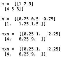
There are two ways of calculating the multiplication of two matrices, the first is by using “*” and the second by using a function named multiply() and passing matrices to it as parameters.

import numpy
m = np.array([[1,2,3],[4,5,6]])
print('m = ', m, 'n')
n = m * 0.25
print('n = ', n, 'n')
print('mxn = ',m * n, 'n')
print('mxn = ',np.multiply(m, n))

For calculating the dot product of two matrices a function named matmul() is used where we pass the matrices as parameters.

import numpy as np
a = np.array([[1,2,3,4],[5,6,7,8]])
print('a = ', a, 'n')
b = np.array([[1,2,3],[4,5,6],[7,8,9],[10,11,12]])
print('b = ', b, 'n')
c = np.matmul(a, b)
print('m.n = ', c, 'n')

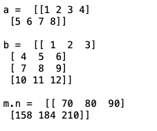
Keep in mind that matrices shapes should be compatible otherwise you would face the shape error.

Matrix Transpose using NumPy

Now there is only one thing left to discuss which is calculating the transpose of a matrix, this is the most used operation while working on the Neural Networks math. Transpose is an operation of converting a matrix into another matrix such that rows from the original matrix are columns in another and columns in the original one are rows in the resultant matrix.

 

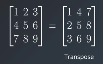
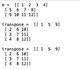
To calculate the transpose of any matrix you can use the transpose function of the NumPy or you can use “.T” to do the same.

import numpy 
m = np.array([[1,2,3,4], [5,6,7,8], [9,10,11,12]])
print('m = ', m, 'n')
n = m.T
print('transpose = ', n, 'n')
o = m.transpose()
print('transpose = ', o, 'n')

 

 Conclusion

The first step towards learning the Deep Learning technology is to set up the python and virtual environment which I hope you can do now on your own. Setting up an Anaconda environment and creating a virtual environment would give you the confidence and excitement to move further in Deep Learning.

Also, you now have a deeper understanding of what kind of operations are used in Neural Network math. Only going through these concepts would not be enough you would have to practice them with different input shapes and check what outputs or errors you would get. This would help you debug the errors in the future when you would be training your own NN models.

In the next series of lectures, I would be diving deeper into more conceptual and technical concepts so stay tuned to learn something new and exciting.

References:

https://Udacity.com

Thanks for reading this article do like if you have learned something new, feel free to comment See you next time !!! ❤️ 

Gourav Singh 29 Sep 2021

Applied Machine Learning Engineer skilled in Computer Vision/Deep Learning Pipeline Development, creating machine learning models, retraining systems and transforming data science prototypes to production-grade solutions. Consistently optimizes and improves real-time systems by evaluating strategies and testing on real world scenarios.