An Introduction to Random Forest Algorithm for beginners
Overview
Random forests are a supervised Machine learning algorithm that is widely used in regression and classification problems and produces, even without hyperparameter tuning a great result most of the time. It is perhaps the most used algorithm because of its simplicity. It builds a number of decision trees on different samples and then takes the majority vote if it’s a classification problem.
I am assuming you have already read about Decision Trees, if not then no need to worry we’ll read everything from start. In this article, we’ll figure out how the Random Forest algorithm works, how to use it, and the math intuition behind this simple algorithm.
Before learning this algorithm let’s first see what are Ensemble techniques.
Contents
- Ensemble Techniques
-
- Boosting
- Bagging
- What is Random Forest?
- Real-life Analogy
- Understanding Decision Trees
- Gini Index
- Applying Decision Trees on Random Forest
- Steps Involved in Random Forest Algorithm
- OOB (Out of the Bag) Evaluation
- Difference between Random Forest and Decision Trees
- Feature Importance Using Random Forest
- Advantages and Disadvantages of Random Forest
- Implementation of Random Forest
- End Notes
Ensemble Techniques
Suppose you want to purchase a house, will you just walk into society and purchase the very first house you see, or based on the advice of your broker will you buy a house? It’s highly unlikely.
You would likely browse a few web portals, checking for the area, number of bedrooms, facilities, price, etc. You will also probably ask your friends and colleagues for their opinion. In short, you wouldn’t directly reach a conclusion, but will instead make a decision considering the opinions of other people as well.
Ensemble techniques work in a similar manner, it simply combines multiple models. Thus, a collection of models is used to make predictions rather than an individual model and this will increase the overall performance. Let’s understand 2 main ensemble methods in Machine Learning:
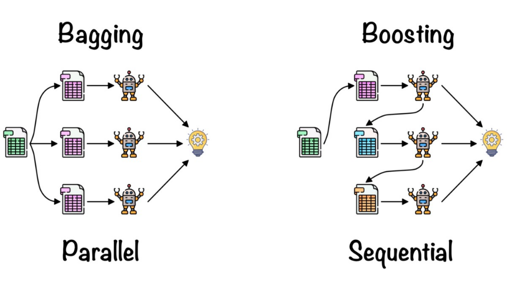
1. Bagging – Suppose we have a dataset, and we make different models on the same dataset and combine it, will it be useful? No right? There is a high chance we’ll get the same results since we are giving the same input. So instead we use a technique called bootstrapping. In this, we create subsets of the original dataset with replacement. The size of the subsets is the same as the size of the original set. Since we do this with replacement so there is a high chance that we provide different data points to our models.
2. Boosting – Suppose any data point in your observation has been incorrectly classified by your 1st model, and then the next (probably all the models), will combine the predictions provide better results? Off-course it’s a big NO.
Boosting technique is a sequential process, where each model tries to correct the errors of the previous model. The succeeding models are dependent on the previous model.
It combines weak learners into strong learners by creating sequential models such that the final model has the highest accuracy. For example, ADA BOOST, XG BOOST.
Random forest works on the bagging principle and now let’s dive into this topic and learn more about how random forest works.
What is the Random Forest Algorithm?
Random Forest is a technique that uses ensemble learning, that combines many weak classifiers to provide solutions to complex problems.
As the name suggests random forest consists of many decision trees. Rather than depending on one tree it takes the prediction from each tree and based on the majority votes of predictions, predicts the final output. Don’t worry if you haven’t read about decision trees, I have that part covered in this article.
Real Life Analogy
Let’s try to understand random forests with the help of an example. Suppose you have to go on a solo trip. You are not sure whether you want to go to a hill station or go somewhere to do some adventure. So, you go to your friend and ask him what does he suggests let’s say friend 1 (F1) tells you to go to a hill station since it’s November already and this will be a great time to have fun there, friend 2 (F2) want’s you to go for adventure. Similarly, all your friends gave you suggestions where you could go on a trip. At last, you can either go to a place of your choice or you decide on a place suggested by most of your friends.
Similarly in Random Forest, we train a number of decision trees, and the class which gets the maximum votes gets to be the final result if it’s a classification problem and average if it’s a regression problem.
Understanding Decision Trees
To know how a random forest algorithm works we need to know Decision Trees which is again a Supervised Machine Learning algorithm used for classification as well as regression problems.
Decision trees use a flowchart like a tree structure to show the predictions that result from a series of feature-based splits. It starts with a root node and ends with a decision made by leaves.
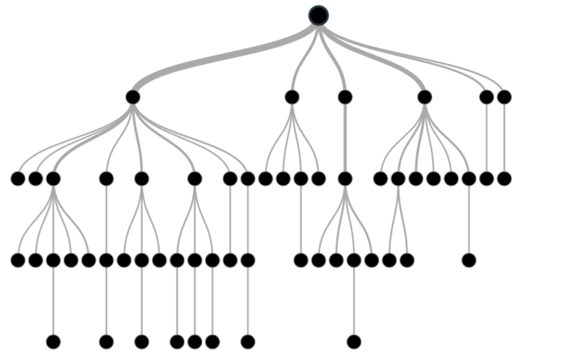
Image 1 – https://wiki.pathmind.com/decision-tree
It consists of 3 components which are the root node, decision node, leaf node. The node from where the population starts dividing is called a root node. The nodes we get after splitting a root node are called decision nodes and the node where further splitting is not possible is called a leaf node. The question comes how do we know which feature will be the root node? In a dataset there can be 100’s of features so how do we decide which feature will be our root node. To answer this question, we need to understand something called the “Gini Index”
What is Gini Index?
To select a feature to split further we need to know how impure or pure that split will be. A pure sub-split means that either you should be getting “yes” or “no”. Suppose this is our dataset.
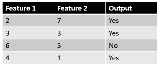
We will see what output we get after splitting, taking each feature as our root node.
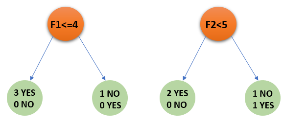
When we take feature 1 as our root node, we get a pure split whereas when we take feature 2, the split is not pure. So how do we know that how much impurity this particular node has? This can be understood with the help of the “Gini Index”.
We basically need to know the impurity of our dataset and we’ll take that feature as the root node which gives the lowest impurity or say which has the lowest Gini index. Mathematically Gini index can be written as:
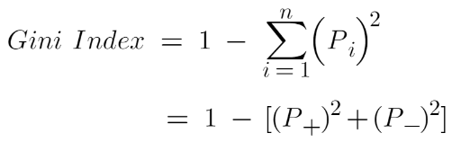
Where P+ is the probability of a positive class and P_ is the probability of a negative class.
Let’s understand this formula with the help of a toy dataset:
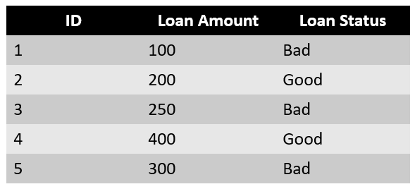
Let’s take Loan Amount as our root node and try to split it:
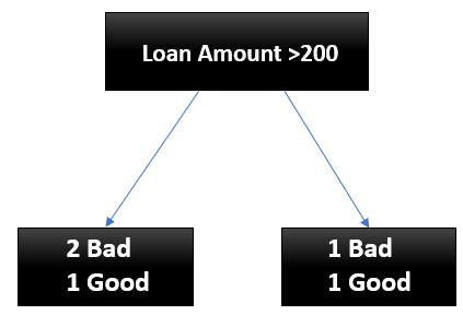
Putting the values of a left split in the formula we get:
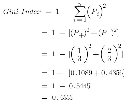
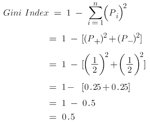
For the right split the Gini index will be:
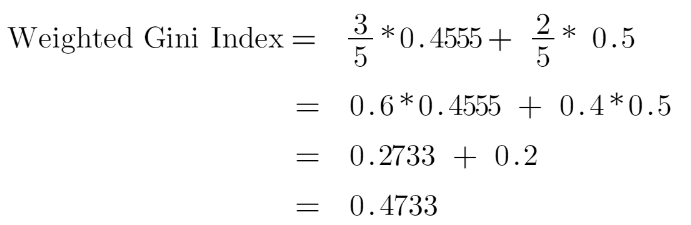
Now we need to calculate the weighted Gini index that is the total Gini index of this split. This can be calculated by:
Similarly, this algorithm will try to find the Gini index of all the splits possible and will choose that feature for the root node which will give the lowest Gini index. The lowest Gini index means low impurity.
You must have heard about another metric called “Entropy” which is also used to measure the impurity of the split. The mathematical formula for entropy is:
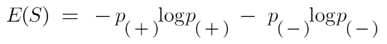
We usually use the Gini index since it is computationally efficient, it takes a shorter period of time for execution because there is no logarithmic term like there is in entropy here. Usually, if you want to do logarithmic calculations it takes some amount of time. That’s why many boosting algorithms use the Gini index as their parameter.
One more important thing to note here is that if there are an equal number of both the classes in a particular node then Gini Index will have its maximum value, which means that the node is highly impure. You can understand this with the help of an example, suppose you have a group of friends, and you all take a vote on which movie to watch. You get 5 votes for ‘lucy’ and 5 for ‘titanic’. Wouldn’t it be harder for you to choose a movie now since both the movies have an equal number of votes, hence we can say that it is a very difficult situation?
Applying Decision trees in Random Forest Algorithm
The main difference between these two is that Random Forest is a bagging method that uses a subset of the original dataset to make predictions and this property of Random Forest helps to overcome Overfitting. Instead of building a single decision tree, Random forest builds a number of DT’s with a different set of observations. One big advantage of this algorithm is that it can be used for classification as well as regression problems.
Steps involved in Random Forest Algorithm
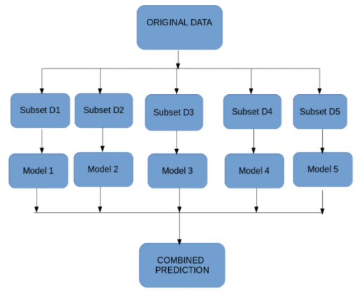
Step-1 – We first make subsets of our original data. We will do row sampling and feature sampling that means we’ll select rows and columns with replacement and create subsets of the training dataset
Step- 2 – We create an individual decision tree for each subset we take
Step-3 – Each decision tree will give an output
Step 4 – Final output is considered based on Majority Voting if it’s a classification problem and average if it’s a regression problem.
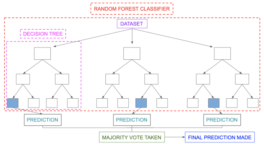
Image Source: https://www.section.io/engineering-education/introduction-to-random-forest-in-machine-learning/
Before proceeding further, we need to know one more important thing that when we grow our decision tree to its depth we get Low Bias and High Variance, we can say that our model will perform perfectly on our training dataset, but it’ll suck when our new datapoint comes into the picture. To tackle this high variance situation, we use random forest where we are combining many decision trees and not just depending on a single DT, this will allow us to lower our variance, and this way we overcome our overfitting problem.
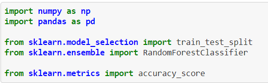
OOB (Out of the bag) Evaluation
We now know how bootstrapping works in random forests. It basically does row sampling and feature sampling with a replacement before training the model. Since sampling is done with replacement, about one-third of the data is not used to train the model and this data is called out of the bag samples. We can evaluate our model on these out-of-bag data points to know how it will perform on the test dataset. Let’s see how we can use this OOB evaluation in python. Let’s import the required libraries:
To explain this, I am taking a small sample that contains data of people having a heart attack:
Python Code:
Next, we’ll separate X and Y and train our model:
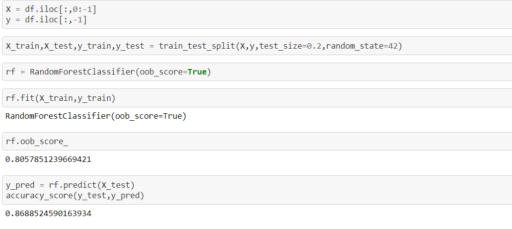
To get the oob evaluation we need to set a parameter called oob_score to TRUE. We can see that the score we get from oob samples, and the test dataset is somewhat the same. In this way, we can use these left-out samples in evaluating our model.
Difference between Decision Tree and Random Forest
|
|
| 1. Decision trees normally suffer from the problem of overfitting if it’s allowed to grow till its maximum depth. | 1. Random forests use the bagging method. It creates a subset of the original dataset, and the final output is based on majority ranking and hence the problem of overfitting is taken care of. |
| 2. A single decision tree is faster in computation. | 2. It is comparatively slower. |
| 3. When a data set with features is taken as input by a decision tree it will formulate some set of rules to do prediction. | 3. Random forest randomly selects observations, builds a decision tree and the average result is taken. It doesn’t use any set of formulas. |
Hence, we can come to a conclusion that random forests are much more successful than decision trees only if the trees are diverse and acceptable.
Feature Importance Using Random Forest
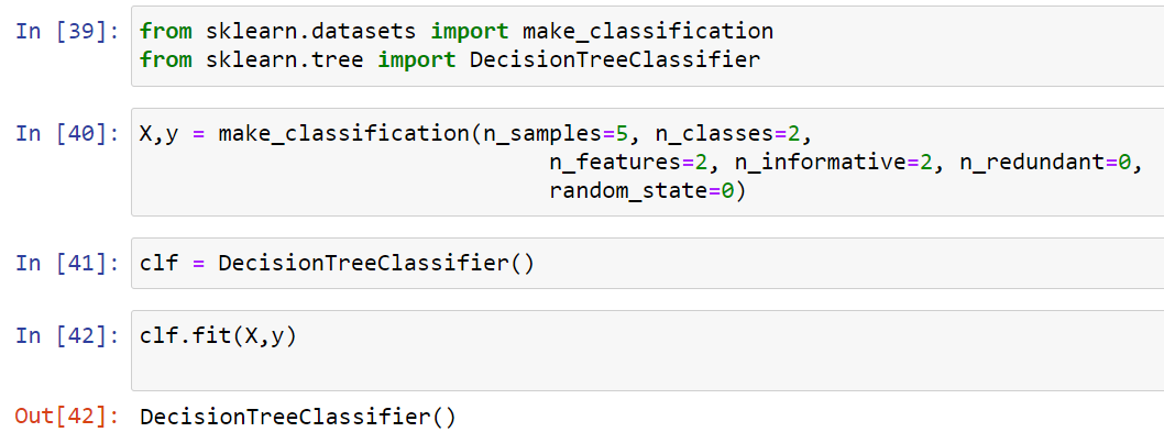
Another great quality of this awesome algorithm is that it can be used for feature selection also. We can use it to know the feature’s importance. To understand how we calculate feature importance in Random Forest we first need to understand how we calculate it using Decision Trees. You need to understand some math’s here but don’t worry I’ll try to explain it in the easiest way possible. Let’s understand it with the help of an example. I am taking 5 rows and 2 columns for simplicity and then fitting DecisionTreeClassifier to this small dataset:
The formula for calculating the feature importance is:
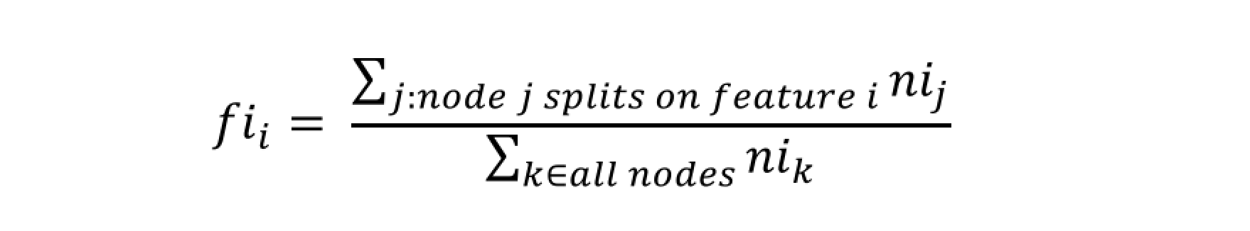
To understand this formula, first, let’s plot the decision tree for the above dataset:
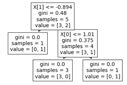
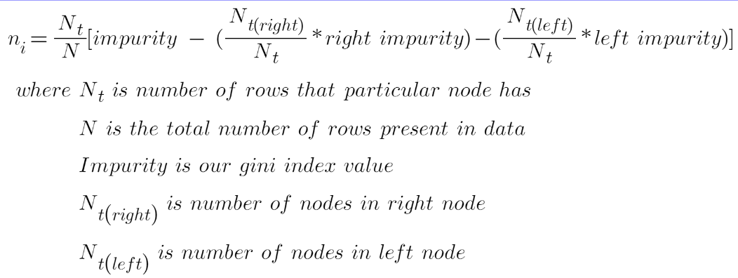
Here we have two columns [0 and 1], to calculate the feature importance of [0] we need to find those nodes where the split happened due to this column [0]. In this dataset, we have only 1 node for column [0] and column [1]. Out of all the nodes, we will find the feature importance of those nodes where the split happened due to column [0] and then divide it by the feature importance of all the nodes. To calculate the importance of a node we will use this formula:
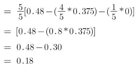
Let’s calculate the feature importance of 1st node in our decision tree.
Our Nt is 5, N is 5, impurity of that node is 0.48, Nt(right) is 4, right impurity is 0.375, Nt(Left) is 1, and left impurity is 0, putting all this information in the above formula we get:
Similarly, we will calculate this for 2nd node:
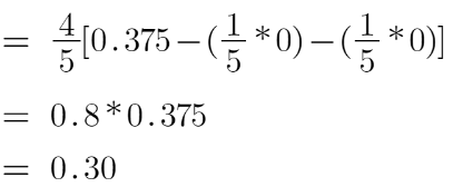
Now let’s calculate the importance of features [0] and [1], This can be calculated as :
![features [0] and [1]](https://editor.analyticsvidhya.com/uploads/7858118.png)
![features [0] and [1] 2](https://editor.analyticsvidhya.com/uploads/2549422.png)
Hence for the feature [0], the feature importance is 0.625 and for [1] it is 0.375.
Let’s look at the code how we can implement this whole using random forest:
from sklearn.datasets import make_classification
from sklearn.tree import DecisionTreeClassifier
X,y = make_classification(n_samples=5, n_classes=2,
                               n_features=2, n_informative=2, n_redundant=0,
                               random_state=0)
clf = DecisionTreeClassifier()
clf.fit(X,y)
from sklearn.tree import plot_tree
plot_tree(clf)
To calculate feature importance using Random Forest we just take an average of all the feature importances from each tree. Suppose DT1 gives us [0.324,0.676], for DT2 the feature importance of our features is [1,0] so what random forest will do is calculate the average of these numbers. So, the final output feature importance of column [1] and column [0] is [0.662,0.338] respectively.
Advantages and Disadvantages of Random Forest
One of the greatest benefits of a random forest algorithm is its flexibility. We can use this algorithm for regression as well as classification problems. It can be considered a handy algorithm because it produces better results even without hyperparameter tuning. Also, the parameters are pretty straightforward, they are easy to understand and there are also not that many of them.
One of the biggest problems in machine learning is Overfitting. We need to make a generalized model which can get good results on the test data too. Random forest helps to overcome this situation by combining many Decision Trees which will eventually give us low bias and low variance.
The main limitation of random forest is that due to a large number of trees the algorithm takes a long time to train which makes it slow and ineffective for real-time predictions. In general, these algorithms are fast to train but quite slow to create predictions once they are trained. In most real-world applications, the random forest algorithm is fast enough but there can certainly be situations where run-time performance is important and other approaches would be preferred.
Implementation of Random Forest algorithm
1. Let’s import the libraries.
# Importing the required libraries
import pandas as pd
import numpy as np
import matplotlib.pyplot as plt
import seaborn as sns
%matplotlib inline
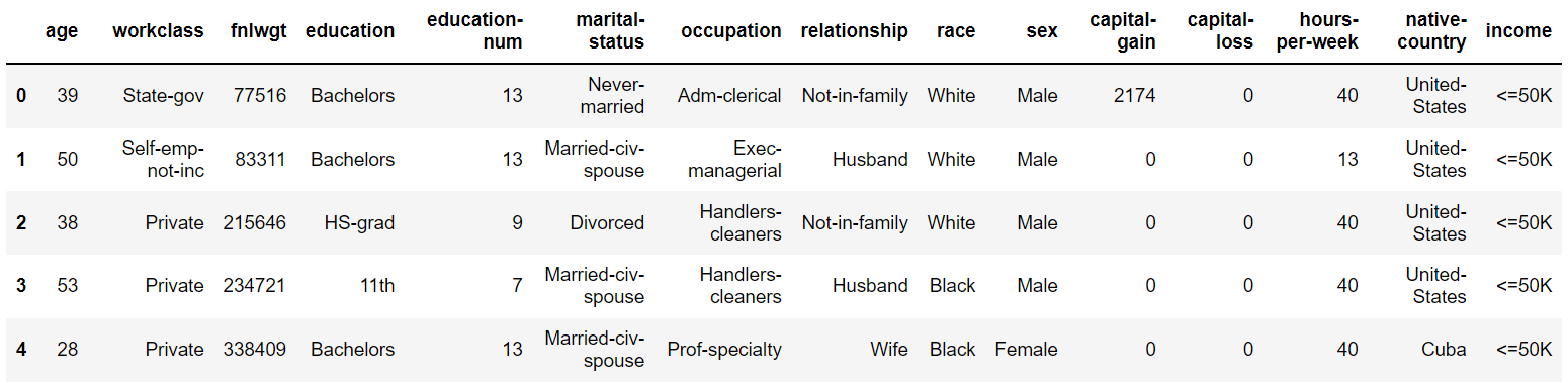
2. Import the dataset
# Reading the csv file and putting it into 'df' object
df = pd.read_csv('heart_v2.csv')
df.head()
3. Putting Feature Variable to X and Target variable to y.
# Putting feature variable to X
X = df.drop('income',axis=1)
# Putting response variable to y
y = df['income']
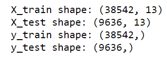
4. Train-Test-Split is performed
# now lets split the data into train and test
from sklearn.model_selection import train_test_split
# Splitting the data into train and test
X_train, X_test, y_train, y_test = train_test_split(X, y, train_size=0.20, random_state=42)
5. Let’s import RandomForestClassifier and fit the data.
from sklearn.ensemble import RandomForestClassifier
classifier_rf = RandomForestClassifier(random_state=42, n_jobs=-1, max_depth=5,
                                       n_estimators=100, oob_score=True)
%%time
classifier_rf.fit(X_train, y_train)

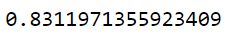
# checking the oob score
classifier_rf.oob_score_
6. Let’s do hyperparameter tuning for Random Forest using GridSearchCV and fit the data.
rf = RandomForestClassifier(random_state=42, n_jobs=-1)
params = {
    'max_depth': [2,3,5,10,20],
    'min_samples_leaf': [5,10,20,50,100,200],
    'n_estimators': [10,25,30,50,100,200]
}
from sklearn.model_selection import GridSearchCV
# Instantiate the grid search model
grid_search = GridSearchCV(estimator=rf,
                           param_grid=params,
                           cv = 4,
                           n_jobs=-1, verbose=1, scoring="accuracy")
%%time
grid_search.fit(X_train, y_train)
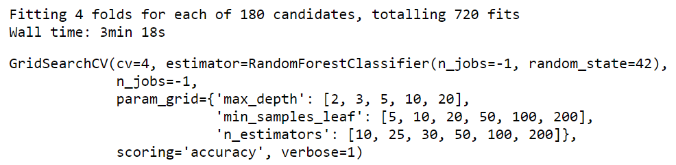
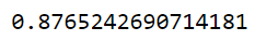
grid_search.best_score_
rf_best = grid_search.best_estimator_
rf_best

From hyperparameter tuning, we can fetch the best estimator as shown. The best set of parameters identified were max_depth=20, min_samples_leaf=5,n_estimators=200
End Notes
In this article, we looked at a very powerful machine learning algorithm. To summarize, we learned about decision trees and random forests. On what basis does the tree split the nodes and how does Random Forest helps us to overcome overfitting. We also know how Random forest help in feature selection.
That is it, you have now mastered this algorithm, all you need is the practice now. Let me know if you have any queries in the comments below.
About the Author
I am an undergraduate student currently in my last year majoring in Statistics (Bachelors of Statistics) and have a strong interest in the field of data science, machine learning, and artificial intelligence. I enjoy diving into data to discover trends and other valuable insights about the data. I am constantly learning and motivated to try new things.
I am open to collaboration and work.
For any doubt and queries, feel free to contact me on Email
Connect with me on LinkedIn and Twitter
Image Sources
- Image 1 – https://wiki.pathmind.com/decision-tree
I am an undergraduate student currently in my last year majoring in Statistics (Bachelors of Statistics) and have a strong interest in the field of data science, machine learning, and artificial intelligence. I enjoy diving into data to discover trends and other valuable insights about the data. I am constantly learning and motivated to try new things.


