Emotion Detection using Bidirectional LSTM and Word2Vec

Introduction

Emotion Detection, as the name suggests, means identifying the emotion behind any text or speech. Emotion detection is a must-do task in Natural Language Processing.

• Emotion detection is already implemented in various business tasks. Take an example of Twitter where millions of users tweet and its ML model can read all posts and can classify the emotion behind tweets.
• Take an example of Amazon where sentiment models classify reviews as positive, negative, and neutral, based on that Amazon gets to know if the product is good or not.

In this article, we will focus on the emotion detection of text data.

There are several ways to perform emotion detection. In this article, you will be using Bidirectional LSTM along with word2vec for better results.

This article assumes that the reader has basic knowledge about CNN & RNN.

RNN (recurrent neural network) is a type of neural network that is generally used to develop speech and text-related models like speech recognition and natural language processing models. Recurrent neural networks remember the sequence (order) of the data and use these data patterns to give predictions.

Bi-LSTM Networks

Bidirectional long-short term memory (Bi-LSTM) is a Neural Network architecture where makes use of information in both directions forward(past to future) or backward (future to past).

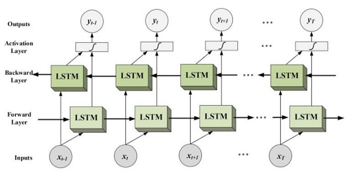
As you see in the image the flow of information from backward and forward layers. Bidirectional LSTM is used where the sequence to sequence tasks are needed. This kind of network is used in text classification, speech recognition, and forecasting models. for more information read here.

In this article, we would be mainly focusing on the implementation part rather than a theoretical one.

Requirement: GPU supported python environment

Loading the Data for Emotion Detection

The dataset used in this article can be downloaded from here. the dataset contains 3 files, train file, test file, Val file.

let’s start with loading our textual data in a data frame, you can do the same using the following code.

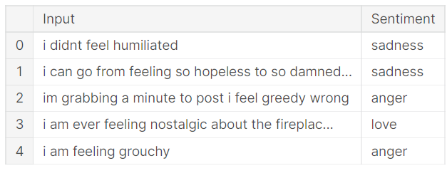
df_train has 16000 rows and 2 columns, df_test & df_val have 2000 rows and 2 columns. Now Let’s check the category-wise distribution of data.

sns.countplot(df_train.Sentiment)
plt.show()

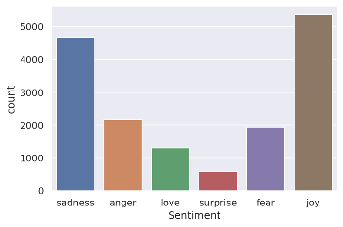
the category Surprise has the least data sample, you can make data balanced by balancing all categories either by over-sampling or under-sampling.

Emotion Detection Data Preprocessing

In order to make our text data cleaner we need to perform some text preprocessing.

• removing punctuations (it doesn’t contribute to emotion detection).
• removing stopwords ( i.e. words like the, are, etc. which also does not contribute to the task).
• removing emails, HTML tags, website, and unnecessary links.
• removing contraction of words ( I’m -> I am ).
• normalisation or words ( eating -> eat, playing -> play).

To make text-preprocessing easier I have written a library named text_hammer. let’s look at how it works.

installing and importing text_hammer: 

!pip install text_hammer 
import text_hammer as th

now importing tqdm progress bar and creating a function which takes data-frame to perform preprocessing and return a preprocessed data-frame.

%%time
from tqdm._tqdm_notebook import tqdm_notebook
tqdm_notebook.pandas()

def text_preprocessing(df,col_name):
    column = col_name
    df[column] = df[column].progress_apply(lambda x:str(x).lower())
    df[column] = df[column].progress_apply(lambda x: th.cont_exp(x))

    #you're -> you are; i'm -> i am

    df[column] = df[column].progress_apply(lambda x: th.remove_emails(x))
    df[column] = df[column].progress_apply(lambda x: th.remove_html_tags(x))
    df[column] = df[column].progress_apply(lambda x: th.remove_special_chars(x))
    df[column] = df[column].progress_apply(lambda x: th.remove_accented_chars(x))
    df[column] = df[column].progress_apply(lambda x: th.make_base(x)) #ran -> run,
    return(df)

the method progress_apply() is used when we create a progress bar associated with the method apply().

lambda function takes a sentence and passes it into text_preprocessing methods.

th.make_base() takes a sentence and returns normalized sentence.

th.remove_accented_chars() removes accented characters.

after building text-preprocessing function we need call it on our dataframe. only training data need to be cleaned, not test and validation data

“Input” is the column containing our text data .
calling tEmotionffffext_preprocessing may take time depeding on the data size.

df_cleaned_train = text_preprocessing(df_train, 'Input')

Label Encoding

The sentiment category in our data frame needs to be converted into some numbers in order to pass into the model.

using a dictionary we are encoding our sentiment categories {‘joy’:0,’anger’:1,’love’:2,’sadness’:3,’fear’:4,’surprise’:5}.

df_cleaned_train['Sentiment'] = df_cleaned_train.Sentiment.replace({'joy':0,'anger':1,'love':2,'sadness':3,'fear':4,'surprise':5})
df_test['Sentiment'] = df_test.Sentiment.replace({'joy':0,'anger':1,'love':2,'sadness':3,'fear':4,'surprise':5})
df_val['Sentiment'] = df_val.Sentiment.replace({'joy':0,'anger':1,'love':2,'sadness':3,

we have encoded our category by assigning them numbers now it’s time to convert categories into categorical data.

from keras.utils import to_categorical
y_train = to_categorical(df_cleaned_train.Sentiment.values)
y_test = to_categorical(df_test.Sentiment.values)
y_val = to_categorical(df_val.Sentiment.values)

y_val, y_test, y_train are now a binary matrix that will be passed in our model.

Tokenization

As you see we have converted our sentiment labels into some numbers and then into a binary matrix, but what about our text data? we can’t pass text directly to our model.

So it’s time to convert our text corpus into some integer numbers.

Tokenizer class converts a sentence into an array of numbers by assigning them numbers based on their frequency.

from keras.preprocessing.text import Tokenizernum_words = 10000 # this means 10000 unique words can be taken 
tokenizer=Tokenizer(num_words,lower=True)
df_total = pd.concat([df_cleaned_train['Input'], df_test.Input], axis = 0)
tokenizer.fit_on_texts(df_total)

Only the top “num_words” i.e. most frequent words will be taken into account. Only words known by the tokenizer will be taken into account hence we have concatenated our train and test data to increase the vocabulary for the tokenizer.

The method fit_on_texts() fits the text data to the tokenizer. It takes a list of sentences.

from keras.preprocessing.sequence import pad_sequences

X_train=tokenizer.texts_to_sequences(df_cleaned_train['Input']) # this converts texts into some numeric sequences 
X_train_pad=pad_sequences(X_train,maxlen=300,padding='post') # this makes the length of all numeric sequences equal 
X_test = tokenizer.texts_to_sequences(df_test.Input)
X_test_pad = pad_sequences(X_test, maxlen = 300, padding = 'post')
X_val = tokenizer.texts_to_sequences(df_val.Input)
X_val_pad = pad_sequences(X_val, maxlen = 300, padding = 'post')

texts_to_sequence() takes a list of sentences and converts them into a sequence of numbers.

Since in our data different sentences have different lengths, it means the number sequence made by texts_to_sequence will also have different lengths. in order to pass them in our model, we must make all of them of the same length.

pad_sequences is used to ensure that all sequences in a list have the same length. By default, this is done by padding 0 at the beginning/end (pre, post) of each sequence until each sequence has the same length as the longest sequence. If in case the sequence length is greater than maxlen, it also trims from the end.

x_train_pad.shape is now (16000,300).

x_test_pad.shape is now (2000,300).

x_val_pad.shape is now (2000,300).

now we have lists containing our sequences of the same length.

Word2Vec

Before proceeding to the next step, you need to look back to the last step there is one problem in our approach.

Let’s say we have words (‘love’, ‘affection’,’ like’) these words have
the same meaning but according to our tokenizer these words are treated
differently. we need to create a relationship between all those words
which are interrelated.

Here word embedding comes into play, for more understanding read here.

We are going to use glove-wiki-gigaword-100 which is trained on Wikipedia data and maps a word into an array of length 100. we also have glove-wiki-gigaword-300 which gives a better result but it’s computationally heavy because of higher dimension.

Loading the pertained glove vector using the gensim library.

#pip install gensim
import gensim.downloader as api
glove_gensim  = api.load('glove-wiki-gigaword-100') #100 dimension

More dimension means more deep meaning of words but it may take a longer time to download.

Now map the vocabulary learned by the tokenizer and create a weight matrix.

vector_size = 100
gensim_weight_matrix = np.zeros((num_words ,vector_size))
gensim_weight_matrix.shape

for word, index in tokenizer.word_index.items():
    if index < num_words: # since index starts with zero 
        if word in glove_gensim.wv.vocab:
            gensim_weight_matrix[index] = glove_gensim[word]
        else:
            gensim_weight_matrix[index] = np.zeros(100)

tokenizer.word_index.items() returns a dictionary of unique words as key and frequency as value.

• Iterating the unique words and finding the corresponding word in glove_gensim.wv.vocab
• glove_gensim[‘DOG’] returns the word vector for ‘DOG’.
• If a word is found in glove vocabulary then return the corresponding vector and append it in gensim_weight_matrix.
• gensim_weight_matrix must have the size of (number of unique words, glove_dimension).

Emotion Detection Model Building

So far we preprocessed our data, converted our y_label into categorical data, mapped our vocabulary into the vector using word2vec.

It’s time to design our Bi-LSTM model.

Importing libraries needed.

from tensorflow.keras.models import Sequential 
from tensorflow.keras.layers import Dense, LSTM, Embedding,Bidirectional
import tensorflow
from tensorflow.compat.v1.keras.layers import CuDNNLSTM
from tensorflow.keras.layers import Dropout

Embedding Layer: we already have created a word-embedding matrix. to feed our word_embedding matrix in our training we would use an embedding layer.

There are 3 parameters in embedding layers.

• input_dim : Vocabulary Size( number of unique words for training)
• output_dim : Length of the vector for each word(embedding dimension)
• input_length : Maximum length of a sequence
• trainable : It’s False, which means it will only use a given weight matrix,

EMBEDDING_DIM = 100
class_num = 6
model = Sequential()
model.add(Embedding(input_dim = num_words,
 output_dim = EMBEDDING_DIM,
 input_length= X_train_pad.shape[1],
 weights = [gensim_weight_matrix],trainable = False))model.add(Dropout(0.2))
model.add(Bidirectional(CuDNNLSTM(100,return_sequences=True)))
model.add(Dropout(0.2))
model.add(Bidirectional(CuDNNLSTM(200,return_sequences=True)))
model.add(Dropout(0.2))
model.add(Bidirectional(CuDNNLSTM(100,return_sequences=False)))
model.add(Dense(class_num, activation = ‘softmax’))
model.compile(loss = ‘categorical_crossentropy’, optimizer = ‘adam’,metrics = ‘accuracy’)

• EMBEDDING_DIM = 100 means the embedding layer will create a vector in 100 dimensions.
• While Stacking RNN, the former RNN layers should be set return_sequences to True so that the following RNN layer layers can have the full sequence as input.
• class_num = 6 since we have 6 categories to classify.

Defining Callbacks

In order to train efficiently, we defined some callbacks.

#EarlyStopping and ModelCheckpoint
from keras.callbacks import EarlyStopping, ModelCheckpoint
es = EarlyStopping(monitor = 'val_loss', mode = 'min', verbose = 1, patience = 5)
mc = ModelCheckpoint('./model.h5', monitor = 'val_accuracy', mode = 'max', verbose = 1, save_best_only = True)

• EarlyStopping stops the training after some patience if no further improvement is observed or if training loss decreases and validation loss increases after a certain point.
• ModelChckpoint saves the model checkpoint.

Training model

Now we are ready to train our designed model.

history_embedding = model.fit(X_train_pad, y_train, 
                                epochs = 25, batch_size = 120, 
                                validation_data=(X_val_pad, y_val),
                                verbose = 1, callbacks= [es, mc]  )

history_embedding keeps the history of model training.

Plotting the History

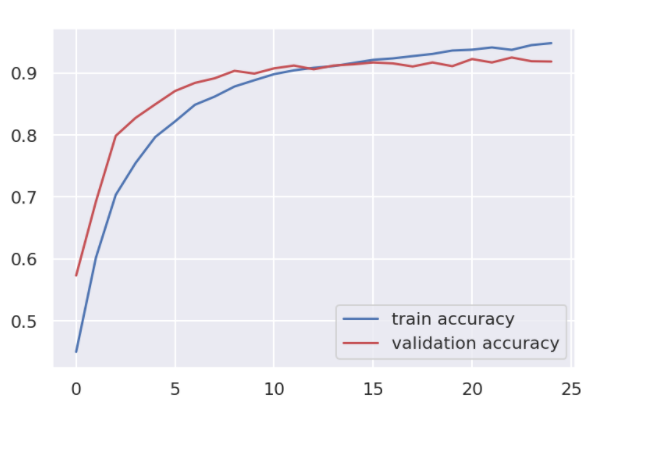
Using training history analyzing the model performance. 

plt.plot(history_embedding.history['accuracy'],c='b',label='train accuracy')
plt.plot(history_embedding.history['val_accuracy'],c='r',label='validation accuracy')
plt.legend(loc='lower right')
plt.show()

Test the Emotion Detection Model

We have prepared X_test_pad for testing purposes, it’s time to test on it.

np.argmax returns the index of maximum probability.

y_pred =   np.argmax(model.predict(X_test_pad), axis  =  1)
y_true = np.argmax(y_test, axis = 1)
from sklearn import metrics
print(metrics.classification_report(y_pred, y_true))

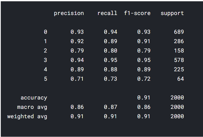
wow! it really performed well, as you see this is the result we got using our test data.

Conclusion

This is how you can create an emotion detection model, let’s recheck the whole pipeline again:

1. Take the input text.
2. Use tokenizer converts into integer sequence.
3. Use pad_sequence to make sequence length equal to the length used for training.
4. Now pass the padded_sequence to model and call predict method, it will give you class index.
5. Using the dictionary we defined earlier change the class index to the class label.

you can improve results further by using the BERT State of the Art model and by using word embeddings of higher dimensions ie 300 you can improve further.

code used in this article can be downloaded from this link.

Thanks for reading the article, please share if you liked this article.