Guide on Support Vector Machine (SVM) Algorithm
Introduction
SVM is a powerful supervised algorithm that works best on smaller datasets but on complex ones. Support Vector Machine, abbreviated as SVM can be used for both regression and classification tasks, but generally, they work best in classification problems. They were very famous around the time they were created, during the 1990s, and keep on being the go-to method for a high-performing algorithm with a little tuning.
By now, I hope you’ve now mastered Decision Trees, Random Forest, Naïve Bayes, K-nearest neighbor, and Ensemble Modelling techniques. If not, I would suggest you take out a few minutes and read about them as well.
In this article, I will explain to you What is SVM, how SVM Algorithm works, and the math intuition behind this crucial ML algorithm.
This article was published as a part of the Data Science Blogathon!
Table of contents
- What is a Support Vector Machine(SVM)?
- Logistic Regression vs Support Vector Machine (SVM)
- Types of Support Vector Machine (SVM) Algorithms
- Important Terms
- How Does Support Vector Machine Work?
- Mathematical Intuition Behind Support Vector Machine
- Margin in Support Vector Machine
- Optimization F unction and its Constraints
- Kernels in Support Vector Machine
- Implementation and hyperparameter tuning of Support Vector Machine in Python
- Conclusion
- Frequently Asked Questions
What is a Support Vector Machine(SVM)?
It is a supervised machine learning problem where we try to find a hyperplane that best separates the two classes. Note: Don’t get confused between SVM and logistic regression. Both the algorithms try to find the best hyperplane, but the main difference is logistic regression is a probabilistic approach whereas support vector machine is based on statistical approaches.
Now the question is which hyperplane does it select? There can be an infinite number of hyperplanes passing through a point and classifying the two classes perfectly. So, which one is the best?
Well, SVM does this by finding the maximum margin between the hyperplanes that means maximum distances between the two classes.
Logistic Regression vs Support Vector Machine (SVM)
Depending on the number of features you have you can either choose Logistic Regression or SVM.
SVM works best when the dataset is small and complex. It is usually advisable to first use logistic regression and see how does it performs, if it fails to give a good accuracy you can go for SVM without any kernel (will talk more about kernels in the later section). Logistic regression and SVM without any kernel have similar performance but depending on your features, one may be more efficient than the other.
Types of Support Vector Machine (SVM) Algorithms
- Linear SVM: When the data is perfectly linearly separable only then we can use Linear SVM. Perfectly linearly separable means that the data points can be classified into 2 classes by using a single straight line(if 2D).
- Non-Linear SVM: When the data is not linearly separable then we can use Non-Linear SVM, which means when the data points cannot be separated into 2 classes by using a straight line (if 2D) then we use some advanced techniques like kernel tricks to classify them. In most real-world applications we do not find linearly separable datapoints hence we use kernel trick to solve them.
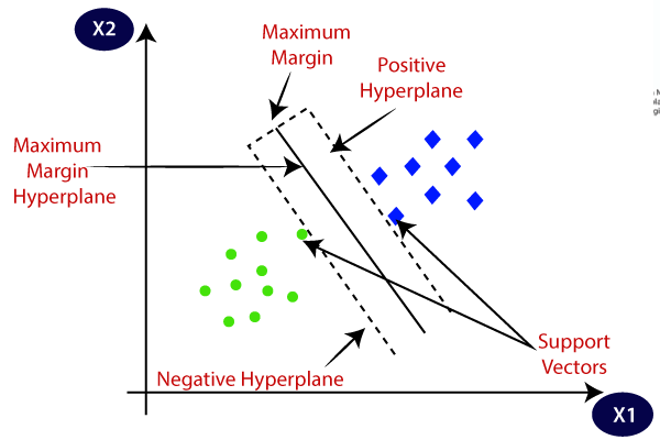
Important Terms
Now let’s define two main terms which will be repeated again and again in this article:
- Support Vectors: These are the points that are closest to the hyperplane. A separating line will be defined with the help of these data points.
- Margin: it is the distance between the hyperplane and the observations closest to the hyperplane (support vectors). In SVM large margin is considered a good margin. There are two types of margins hard margin and soft margin. I will talk more about these two in the later section.
How Does Support Vector Machine Work?
SVM is defined such that it is defined in terms of the support vectors only, we don’t have to worry about other observations since the margin is made using the points which are closest to the hyperplane (support vectors), whereas in logistic regression the classifier is defined over all the points. Hence SVM enjoys some natural speed-ups.
Let’s understand the working of SVM using an example. Suppose we have a dataset that has two classes (green and blue). We want to classify that the new data point as either blue or green.
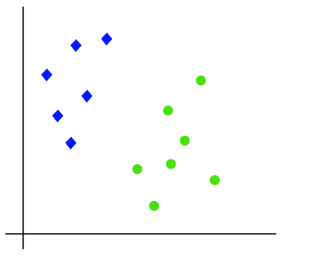
To classify these points, we can have many decision boundaries, but the question is which is the best and how do we find it? NOTE: Since we are plotting the data points in a 2-dimensional graph we call this decision boundary a straight line but if we have more dimensions, we call this decision boundary a “hyperplane”
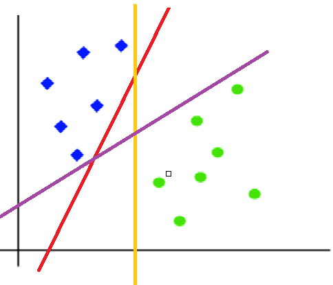
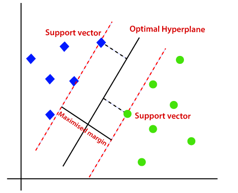
The best hyperplane is that plane that has the maximum distance from both the classes, and this is the main aim of SVM. This is done by finding different hyperplanes which classify the labels in the best way then it will choose the one which is farthest from the data points or the one which has a maximum margin.
Mathematical Intuition Behind Support Vector Machine
Many people skip the math intuition behind this algorithm because it is pretty hard to digest. Here in this section, we’ll try to understand each and every step working under the hood. SVM is a broad topic and people are still doing research on this algorithm. If you are planning to do research, then this might not be the right place for you.
Here we will understand only that part that is required in implementing this algorithm. You must have heard about the primal formulation, dual formulation, Lagranges multiplier etc. I am not saying these topics aren’t important, but they are more important if you are planning to do research in this area. Let’s move ahead and see the magic behind this algorithm.
Before getting into the nitty-gritty details of this topic first let’s understand what a dot product is.
Understanding Dot-Product
We all know that a vector is a quantity that has magnitude as well as direction and just like numbers we can use mathematical operations such as addition, multiplication. In this section, we will try to learn about the multiplication of vectors which can be done in two ways, dot product, and cross product. The difference is only that the dot product is used to get a scalar value as a resultant whereas cross-product is used to obtain a vector again.
The dot product can be defined as the projection of one vector along with another, multiply by the product of another vector.
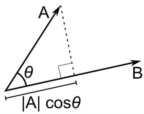
Image 2
Here a and b are 2 vectors, to find the dot product between these 2 vectors we first find the magnitude of both the vectors and to find magnitude we use the Pythagorean theorem or the distance formula.
After finding the magnitude we simply multiply it with the cosine angle between both the vectors. Mathematically it can be written as:
A . B = |A| cosθ * |B|
Where |A| cosθ is the projection of A on B
And |B| is the magnitude of vector B
Now in SVM we just need the projection of A not the magnitude of B, I’ll tell you why later. To just get the projection we can simply take the unit vector of B because it will be in the direction of B but its magnitude will be 1. Hence now the equation becomes:
A.B = |A| cosθ * unit vector of B
Now let’s move to the next part and see how we will use this in SVM.
Use of Dot Product in SVM
Consider a random point X and we want to know whether it lies on the right side of the plane or the left side of the plane (positive or negative).
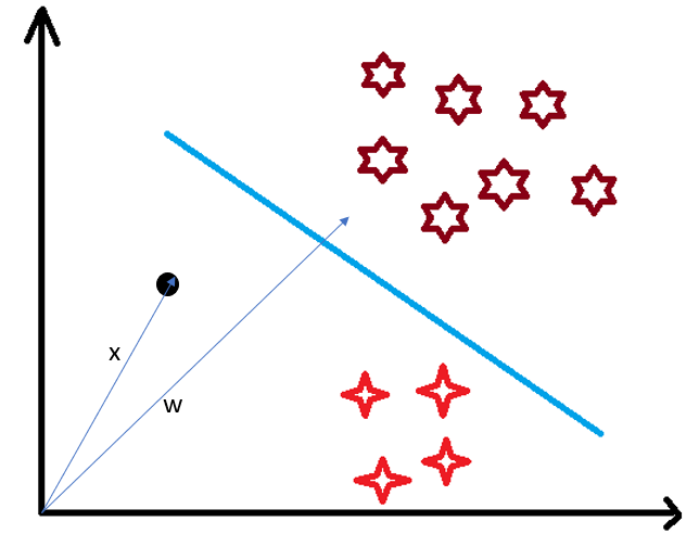
To find this first we assume this point is a vector (X) and then we make a vector (w) which is perpendicular to the hyperplane. Let’s say the distance of vector w from origin to decision boundary is ‘c’. Now we take the projection of X vector on w.
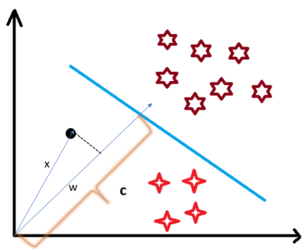
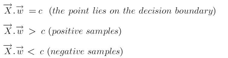
We already know that projection of any vector or another vector is called dot-product. Hence, we take the dot product of x and w vectors. If the dot product is greater than ‘c’ then we can say that the point lies on the right side. If the dot product is less than ‘c’ then the point is on the left side and if the dot product is equal to ‘c’ then the point lies on the decision boundary.
You must be having this doubt that why did we take this perpendicular vector w to the hyperplane? So what we want is the distance of vector X from the decision boundary and there can be infinite points on the boundary to measure the distance from. So that’s why we come to standard, we simply take perpendicular and use it as a reference and then take projections of all the other data points on this perpendicular vector and then compare the distance.
In SVM we also have a concept of margin. In the next section, we will see how we find the equation of a hyperplane and what exactly do we need to optimize in SVM.
Margin in Support Vector Machine
We all know the equation of a hyperplane is w.x+b=0 where w is a vector normal to hyperplane and b is an offset.
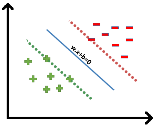
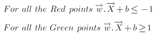
To classify a point as negative or positive we need to define a decision rule. We can define decision rule as:
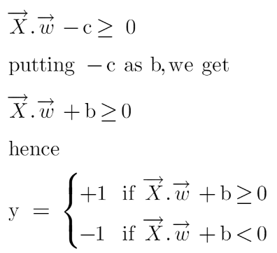
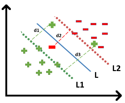
If the value of w.x+b>0 then we can say it is a positive point otherwise it is a negative point. Now we need (w,b) such that the margin has a maximum distance. Let’s say this distance is ‘d’.
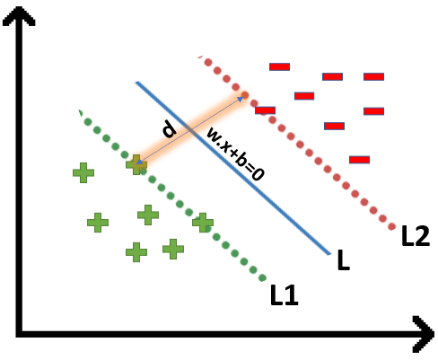
To calculate ‘d’ we need the equation of L1 and L2. For this, we will take few assumptions that the equation of L1 is w.x+b=1 and for L2 it is w.x+b=-1.
Now the question comes
- Why the magnitude is equal, why didn’t we take 1 and -2?
- Why did we only take 1 and -1, why not any other value like 24 and -100?
- Why did we assume this line?
Let’s try to answer these questions
- We want our plane to have equal distance from both the classes that means L should pass through the center of L1 and L2 that’s why we take magnitude equal.
- Let’s say the equation of our hyperplane is 2x+y=2, we observe that even if we multiply the whole equation with some other number the line doesn’t change (try plotting on a graph). Hence for mathematical convenience, we take it as 1.
- Now the main question is exactly why there’s a need to assume only this line? To answer this, I’ll try to take the help of graphs.
Suppose the equation of our hyperplane is 2x+y=2:
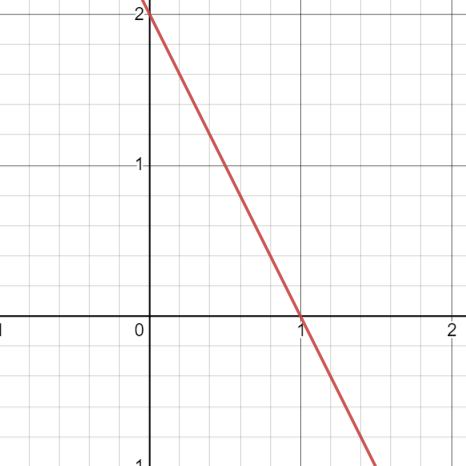
Let’s create margin for this hyperplane,
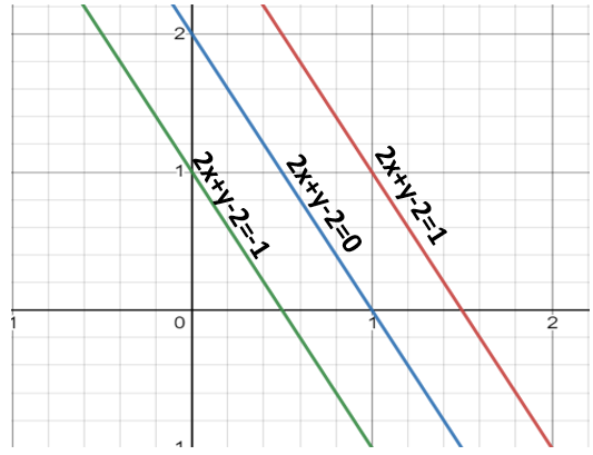
If you multiply these equations by 10, we will see that the parallel line (red and green) gets closer to our hyperplane. For more clarity look at this graph (https://www.desmos.com/calculator/dvjo3vacyp)
We also observe that if we divide this equation by 10 then these parallel lines get bigger. Look at this graph (https://www.desmos.com/calculator/15dbwehq9g).
By this I wanted to show you that the parallel lines depend on (w,b) of our hyperplane, if we multiply the equation of hyperplane with a factor greater than 1 then the parallel lines will shrink and if we multiply with a factor less than 1, they expand.
We can now say that these lines will move as we do changes in (w,b) and this is how this gets optimized. But what is the optimization function? Let’s calculate it.
We know that the aim of SVM is to maximize this margin that means distance (d). But there are few constraints for this distance (d). Let’s look at what these constraints are.
Optimization Function and its Constraints
In order to get our optimization function, there are few constraints to consider. That constraint is that “We’ll calculate the distance (d) in such a way that no positive or negative point can cross the margin line”. Let’s write these constraints mathematically:
Rather than taking 2 constraints forward, we’ll now try to simplify these two constraints into 1. We assume that negative classes have y=-1 and positive classes have y=1.
We can say that for every point to be correctly classified this condition should always be true:
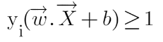
Suppose a green point is correctly classified that means it will follow w.x+b>=1, if we multiply this with y=1 we get this same equation mentioned above. Similarly, if we do this with a red point with y=-1 we will again get this equation. Hence, we can say that we need to maximize (d) such that this constraint holds true.
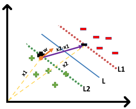
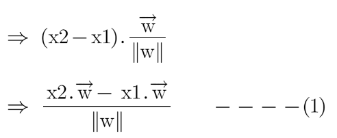
We will take 2 support vectors, 1 from the negative class and 2nd from the positive class. The distance between these two vectors x1 and x2 will be (x2-x1) vector. What we need is, the shortest distance between these two points which can be found using a trick we used in the dot product. We take a vector ‘w’ perpendicular to the hyperplane and then find the projection of (x2-x1) vector on ‘w’. Note: this perpendicular vector should be a unit vector then only this will work. Why this should be a unit vector? This has been explained in the dot-product section. To make this ‘w’ a unit vector we divide this with the norm of ‘w’.
Finding Projection of a Vector on Another Vector Using Dot Product
We already know how to find the projection of a vector on another vector. We do this by dot-product of both vectors. So let’s see how
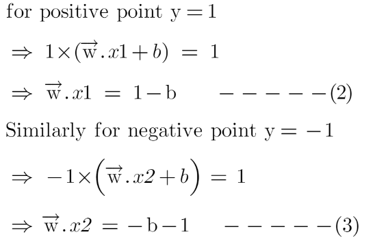
Since x2 and x1 are support vectors and they lie on the hyperplane, hence they will follow yi* (2.x+b)=1 so we can write it as:
Putting equations (2) and (3) in equation (1) we get:
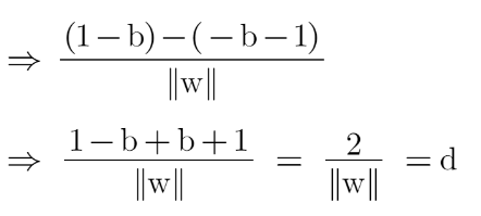
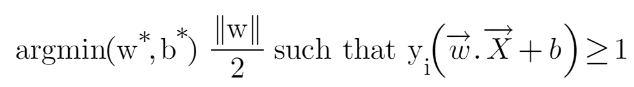
Hence the equation which we have to maximize is:
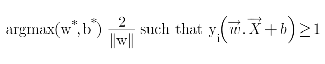
We have now found our optimization function but there is a catch here that we don’t find this type of perfectly linearly separable data in the industry, there is hardly any case we get this type of data and hence we fail to use this condition we proved here. The type of problem which we just studied is called Hard Margin SVM now we shall study soft margin which is similar to this but there are few more interesting tricks we use in Soft Margin SVM.
Soft Margin SVM
In real-life applications, we rarely encounter datasets that are perfectly linearly separable. Instead, we often come across datasets that are either nearly linearly separable or entirely non-linearly separable. Unfortunately, the trick demonstrated above for linearly separable datasets is not applicable in these cases. This is where Support Vector Machines (SVM) come into play. These are a powerful tool in machine learning that can effectively handle both almost linearly separable and non-linearly separable datasets, providing a robust solution to classification problems in diverse real-world scenarios.
To tackle this problem what we do is modify that equation in such a way that it allows few misclassifications that means it allows few points to be wrongly classified.
We know that max[f(x)] can also be written as min[1/f(x)], it is common practice to minimize a cost function for optimization problems; therefore, we can invert the function.
To make a soft margin equation we add 2 more terms to this equation which is zeta and multiply that by a hyperparameter ‘c’
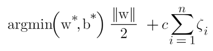
For all the correctly classified points our zeta will be equal to 0 and for all the incorrectly classified points the zeta is simply the distance of that particular point from its correct hyperplane that means if we see the wrongly classified green points the value of zeta will be the distance of these points from L1 hyperplane and for wrongly classified redpoint zeta will be the distance of that point from L2 hyperplane.
So now we can say that our that are SVM Error = Margin Error + Classification Error. The higher the margin, the lower would-be margin error, and vice versa.
Let’s say you take a high value of ‘c’ =1000, this would mean that you don’t want to focus on margin error and just want a model which doesn’t misclassify any data point.
Look at the figure below:
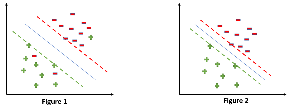
If someone asks you which is a better model, the one where the margin is maximum and has 2 misclassified points or the one where the margin is very less, and all the points are correctly classified?
Well, there’s no correct answer to this question, but rather we can use SVM Error = Margin Error + Classification Error to justify this. If you don’t want any misclassification in the model then you can choose figure 2. That means we’ll increase ‘c’ to decrease Classification Error but if you want that your margin should be maximized then the value of ‘c’ should be minimized. That’s why ‘c’ is a hyperparameter and we find the optimal value of ‘c’ using GridsearchCV and cross-validation.
Kernels in Support Vector Machine
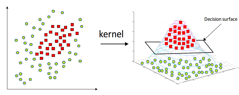
The most interesting feature of SVM is that it can even work with a non-linear dataset and for this, we use “Kernel Trick” which makes it easier to classifies the points. Suppose we have a dataset like this:
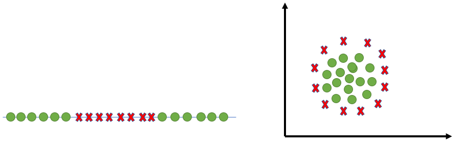
Here we see we cannot draw a single line or say hyperplane which can classify the points correctly. So what we do is try converting this lower dimension space to a higher dimension space using some quadratic functions which will allow us to find a decision boundary that clearly divides the data points. These functions which help us do this are called Kernels and which kernel to use is purely determined by hyperparameter tuning.
Different Kernel Functions
Some kernel functions which you can use in SVM are given below:
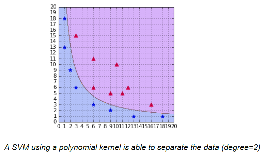
1. Polynomial Kernel
Following is the formula for the polynomial kernel:
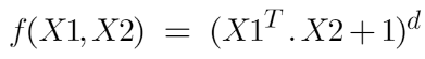
Here d is the degree of the polynomial, which we need to specify manually.
Suppose we have two features X1 and X2 and output variable as Y, so using polynomial kernel we can write it as:
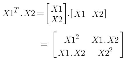
So we basically need to find X12 , X22 and X1.X2, and now we can see that 2 dimensions got converted into 5 dimensions.
2. Sigmoid Kernel
We can use it as the proxy for neural networks. Equation is:
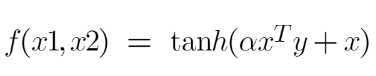
It is just taking your input, mapping them to a value of 0 and 1 so that they can be separated by a simple straight line.
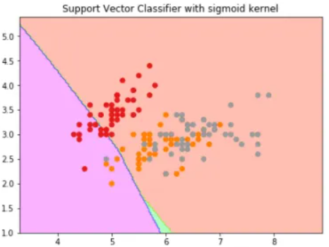
Image Source: https://dataaspirant.com/svm-kernels/#t-1608054630725
3. RBF Kernel
What it actually does is to create non-linear combinations of our features to lift your samples onto a higher-dimensional feature space where we can use a linear decision boundary to separate your classes It is the most used kernel in SVM classifications, the following formula explains it mathematically:
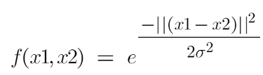
where,
1. ‘σ’ is the variance and our hyperparameter
2. ||X₁ – X₂|| is the Euclidean Distance between two points X₁ and X₂
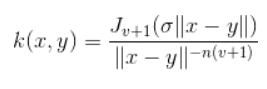
4. Bessel function kernel
It is mainly used for eliminating the cross term in mathematical functions. Following is the formula of the Bessel function kernel:
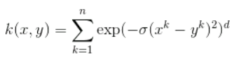
5. Anova Kernel
It performs well on multidimensional regression problems. The formula for this kernel function is:
How to Choose the Right Kernel?
I am well aware of the fact that you must be having this doubt about how to decide which kernel function will work efficiently for your dataset. It is necessary to choose a good kernel function because the performance of the model depends on it.
Choosing a kernel totally depends on what kind of dataset are you working on. If it is linearly separable then you must opt. for linear kernel function since it is very easy to use and the complexity is much lower compared to other kernel functions. I’d recommend you start with a hypothesis that your data is linearly separable and choose a linear kernel function.
You can then work your way up towards the more complex kernel functions. Usually, we use SVM with RBF and linear kernel function because other kernels like polynomial kernel are rarely used due to poor efficiency. But what if linear and RBF both give approximately similar results? Which kernel do we choose now?
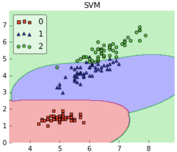
Example
Let’s understand this with the help of an example, for simplicity I’ll only take 2 features that mean 2 dimensions only. In the figure below I have plotted the decision boundary of a linear SVM on 2 features of the iris dataset:
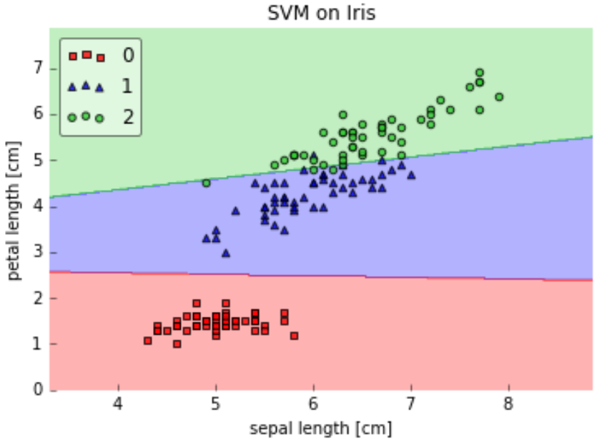
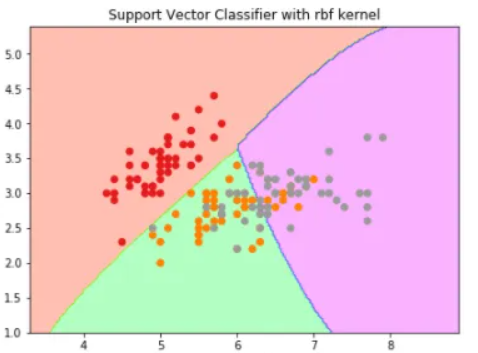
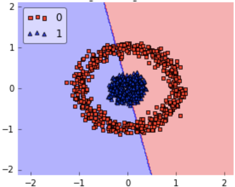
Here we see that a linear kernel works fine on this dataset, but now let’s see how will RBF kernel work.
We can observe that both the kernels give similar results, both work well with our dataset but which one should we choose? Linear SVM is a parametric model. A Parametric Model is a concept used to describe a model in which all its data is represented within its parameters. In short, the only information needed to predict the future from the current value is the parameters.
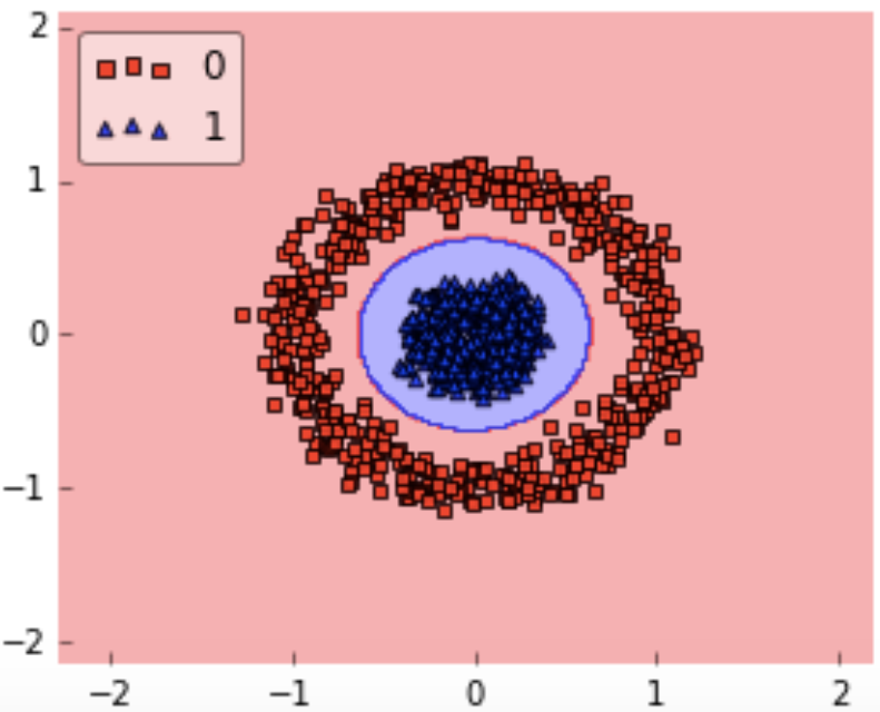
The complexity of the RBF kernel grows as the training data size increases. In addition to the fact that it is more expensive to prepare RBF kernel, we also have to keep the kernel matrix around, and the projection into this “infinite” higher dimensional space where the data becomes linearly separable is more expensive as well during prediction. If the dataset is not linear then using linear kernel doesn’t make sense we’ll get a very low accuracy if we do so.
So for this kind of dataset, we can use RBF without even a second thought because it makes decision boundary like this:
Implementation and hyperparameter tuning of Support Vector Machine in Python
For implementation on a dataset, we will be using the Income Evaluation dataset, which has information about an individual’s personal life and an output of 50K or <=50. The dataset can be found here (https://www.kaggle.com/lodetomasi1995/income-classification)
The task here is to classify the income of an individual when given the required inputs about his personal life.
First, let’s import all required libraries.
# Import all relevant libraries

from sklearn.svm import SVC

import numpy as np

import pandas as pd

from sklearn.preprocessing import StandardScaler

from sklearn.model_selection import train_test_split

from sklearn.metrics import accuracy_score, confusion_matrix

from sklearn import preprocessing

import warnings

warnings.filterwarnings("ignore")

Now let’s read the dataset and look at the columns to understand the information better.

df = pd.read_csv('income_evaluation.csv')

df.head()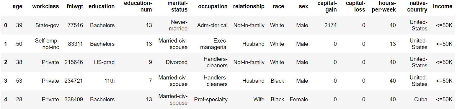
I have already done the data preprocessing part and you can look whole code here. Here my main aim is to tell you how to implement SVM on python.
Now for training and testing our model, the data has to be divided into train and test data.
We will also scale the data to lie between 0 and 1.
# Split dataset into test and train dataNow let’s go ahead with defining the Support vector Classifier along with its hyperparameters. Next, we will fit this model on the training data.
#Define support vector classifier with hyperparameters
X_train, X_test, y_train, y_test = train_test_split(df.drop(‘income’, axis=1),df[‘income’], test_size=0.2)
svc.fit(X_train,y_train)
svc = SVC(random_state=101)
accuracies = cross_val_score(svc,X_train,y_train,cv=5)
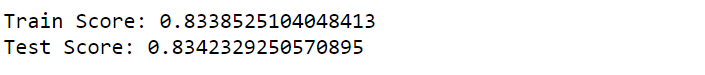
print("Train Score:"np.mean(accuracies))
printf("Test Score:"svc.score(X_test,y_test))The model has been trained and we can now observe the outputs as well.
Below, you can see the accuracy of the test and train dataset
You can even hyper tune your model by the following code:
grid = {

    'C':[0.01,0.1,1,10],

    'kernel' : ["linear","poly","rbf","sigmoid"],

    'degree' : [1,3,5,7],

    'gamma' : [0.01,1]

}

 svm  = SVC ()

svm_cv = GridSearchCV(svm, grid, cv = 5)

svm_cv.fit(X_train,y_train)

print("Best Parameters:",svm_cv.best_params_)

print("Train Score:",svm_cv.best_score_)

print("Test Score:",svm_cv.score(X_test,y_test))
The dataset is pretty big and hence it will take time to get trained, for this reason, I can’t paste the result of the above code here because SVM doesn’t perform well with big datasets, it takes a long time to get trained.
Advantages of SVM
- SVM works better when the data is Linear
- It is more effective in high dimensions
- With the help of the kernel trick, we can solve any complex problem
- SVM is not sensitive to outliers
- Can help us with Image classification
Disadvantages of SVM
- Choosing a good kernel is not easy
- It doesn’t show good results on a big dataset
- The SVM hyperparameters are Cost -C and gamma. It is not that easy to fine-tune these hyper-parameters. It is hard to visualize their impact
Conclusion
In this article, we looked at a very powerful machine learning algorithm, Support Vector Machine in detail. I discussed its concept of working, math intuition behind SVM, implementation in python, the tricks to classify non-linear datasets, Pros and cons, and finally, we solved a problem with the help of SVM.
Frequently Asked Questions
A. SVM algorithm is used for both classification and regression tasks. It finds an optimal hyperplane to separate data points of different classes in a high-dimensional space.
A. SVM is considered one of the best algorithms because it can handle high-dimensional data, is effective in cases with limited training samples, and can handle non-linear classification using kernel functions.
A. The steps of the SVM algorithm involve: (1) selecting the appropriate kernel function, (2) defining the parameters and constraints, (3) solving the optimization problem to find the optimal hyperplane, and (4) making predictions based on the learned model.
A. In machine learning, SVM is used to classify data by finding the optimal decision boundary that maximally separates different classes. It aims to find the best hyperplane that maximizes the margin between support vectors, enabling effective classification even in complex, non-linear scenarios.
The media shown in this article are not owned by Analytics Vidhya and are used at the Author’s discretion.
I am an undergraduate student currently in my last year majoring in Statistics (Bachelors of Statistics) and have a strong interest in the field of data science, machine learning, and artificial intelligence. I enjoy diving into data to discover trends and other valuable insights about the data. I am constantly learning and motivated to try new things.


I think there is a need to validate the code that has been shared here. There are many gaps and errors when executing. Perhaps you could evaluate this on google collaboratory before submitting.
hello sir, you explained SVM very well, thank you
Very well explained. Thank you 🙏
Thanks for your time and effort. It saved me time in searching multiple documents to gain complete insight. This doc is a one-stop solution.
Awesome explanation, Thank You _/\_
Very well explained.Thank you
Very well explained. Every concept has been covered from scratch!!!