A Comprehensive guide to Linear Regression with Perceptron in PyTorch

This article was published as a part of the Data Science Blogathon

Overview of Linear Regression

“Without understanding the engine, building or working with a car is just playing with metal”

This seems to be true in almost all domains of life, without fundamentals; creation and innovation are simply not possible. In this guide, we will understand what is linear regression and how can we implement them using neural networks. The key unit in any neural network – simple or complex are neurons. A neural network with a single neuron is termed a “perceptron”. It was founded by Frank Rosenblatt at Cornell Aeronautical laboratory in 1958. So, it has been around for over 60 years.

During the current rise in deep learning’s applications in the real world, the use of dense neural networks has grown popular with respect to perceptron but that doesn’t say they are still not popular. Here, we will look at the theory as well as the code to build a perceptron to solve a linear regression problem using PyTorch.

Pytorch is a framework designed and developed by Facebook for developing artificial intelligence, machine learning code with ease using tensor computations. It is one of the top 3 most popular frameworks for developing deep learning applications and models. Pytorch is a python package that provides two high-level features:

• Tensor computation (similar to NumPy) with strong support for GPU acceleration.
• Deep neural networks build on a tape-based autograd (One of the ways to calculate automatic gradients) system.

If you wish to read more about Pytorch, here is their official link.

Terminology related to Linear Regression with Perceptron

Tensor: Tensor is an array, a multi-dimensional array that stores the data just like any other data structure. The collection of stored values can be easily accessed through indexing. For better reference, think of tensors in a more imaginative way through this chain of incrementing structure complexity. Scalar –> Vector –> Matrix –> Tensor

Optimization: The process of changing certain values(s) to get a better result altogether.

Loss: The difference between actual and expected output is termed ‘loss’. The term signifies the value that needs to be minimized to get the best-optimized model.

Variable: The input values that we already possess as the data to create a model on are called variables. They are already determined values both at the time of training and inference(evaluation/testing).

Weights: The coefficient values that are attached to the linear equation and optimized during the training to minimize the loss are called weights of a model. These along with bias are also known as model parameters.

Bias: The constant value used in the linear equation to manage the vertical placement of the line over the cartesian plane. It is also termed “y-intercept”(the point where the linear regression line will cut the y-axis)

What is Linear Regression?

One of the earliest machine learning and statistical algorithms to spark the boom in predictive analysis with its simplicity and strong conceptual grounds. Linear regression is a set of words defining themselves. Linear means continuum of any value in a straight-line fashion. It should not have any curves or corners. On the other hand, we have regression, which means “a return to former or less developed state”. We use the word regression because we are looking for regular, reliable patterns that repeat themselves in the long run, and if we were to work with particular values instead of aggregate values, there will be little to no exact relationship between these values because every value includes certain circumstance and its individuality. So to figure out a pattern for approximate prediction for the future, we get down to a less developed state and look at the bigger picture rather detail-oriented.

Now, How do we actually use it in practice?

Linear regression is used to model linear relationships with two or more variables(termed above). One of the variables will always be the dependent variables: the variable that we wish to find future values for, the “target variable“. The other ones (one or more than one) are called independent variables.

Here is the equation for such, where x is our inputs(independent variable), W is the coefficient for independent variable and b is termed as bias (constant).

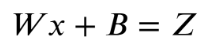
Linear Equation with One Variable

In machine learning, linear regression works by setting the coefficient of independent variable and bias to a random value which during the training period gets optimized by minimizing the difference (termed as a loss) between the results of the linear equation and the target values already provided. This model helps us determine the best possible coefficients for the given data to extract their approximate linear relationship.

What is Perceptron?

The simplest neural network which is nothing but a single neuron is termed a Perceptron. “Neuron” here should not be confused with the biological brain cell, although it inspired the nomenclature of this mathematical model. We don’t need to get in too much detail right here, It will be touched upon in later sections of the article.

A Neuron is nothing but a couple of mathematical functions stacked on top of each other. Here is how it looks like diagrammatically. We have already addressed the first equation in the neuron above. The second equation is a simple functional equation that applies a function on input and produces an output. These functional equations are managed by the engineer in accordance with different problems.

Image link

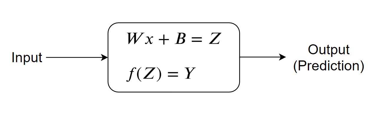
The first equation is the same equation used in simple linear regression with one independent variable and another dependent variable where x is our inputs(independent variable), W and b are coefficients. It is responsible for learning the linear behavior of the data. But, it is not sufficient most of the time to just rely on the linear nature, and understanding of non-linearities becomes critical for an accurate and reasonable model. For such a case, we have this second equation present in the neuron. It’s a function AKA ‘Activation Function’ that depends on the type of problem and your approaches. For making a linear model, we don’t need the activation functions, so we simply avoid their usage.

Code in Pytorch for Linear Regression with Perceptron

Before we start anything, you should know that the python package that we use for PyTorch is: ‘torch’. The first and foremost thing for any project is to figure out what are the essential libraries, packages that will help you in the successful and smart implementation of the project. In our case, other than torch, we will be using Numpy for mathematical computation and Matplotlib for visualization.

1. Importing libraries and Creating Dataset

import numpy as np
import matplotlib.pyplot as plt
import torch

x_train = np.array ([[4.7], [2.4], [7.5], [7.1], [4.3], 
                     [7.8], [8.9], [5.2], [4.59], [2.1], 
                     [8], [5], [7.5], [5], [4],
                     [8], [5.2], [4.9], [3], [4.7], 
                     [4], [4.8], [3.5], [2.1], [4.1]],
                    dtype = np.float32)

y_train = np.array ([[2.6], [1.6], [3.09], [2.4], [2.4], 
                     [3.3], [2.6], [1.96], [3.13], [1.76], 
                     [3.2], [2.1], [1.6], [2.5], [2.2], 
                     [2.75], [2.4], [1.8], [1], [2], 
                     [1.6], [2.4], [2.6], [1.5], [3.1]], 
                    dtype = np.float32)

We created the dataset with some random values as a NumPy array data structure.

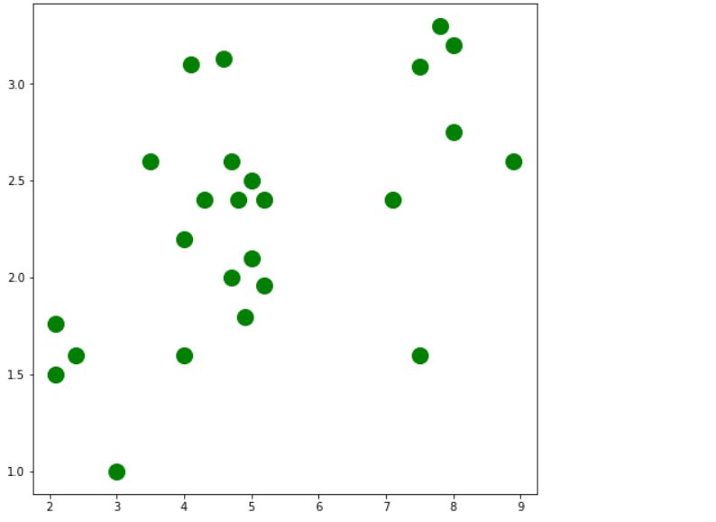
Visualizing the data.

plt.figure(figsize=(8,8))
plt.scatter(x_train, y_train, c='green', s=200, label='Original data')
plt.show()

2. Data preparation and Modelling with Pytorch

Now, the next step is to convert these NumPy arrays into PyTorch tensors(termed above in terminology) because they are the backend data structures that will enable all PyTorch functionalities for further machine learning, deep learning code. So, let us do that.

X_train = torch.from_numpy(x_train) 
Y_train = torch.from_numpy(y_train)
print('requires_grad for X_train: ', X_train.requires_grad)
print('requires_grad for Y_train: ', Y_train.requires_grad)

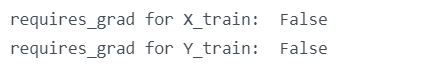
Note: required_grad is the property that manages information in the tensor regarding whether the gradient of the tensor will be calculated during training or not. All the tensors with False value don’t get to store their gradients for their further use.

Modeling in Pytorch

In this article, we are creating the simplest model possible. This model is nothing but the first equation of the neuron which is responsible for determining the linearity in data as mentioned above. Parameters of the model are W1 and b1, which is weight and bias respectively. These parameters are independent in how they turn out to be after getting tuned by the optimizer during training. On the other hand, we have some hyperparameters, which are controllable by the developer and specifically used to manage and direct the process into a more optimized direction during training. Let us have a look at the parameters first.

w1 = torch.rand(input_size, 
                hidden_size, 
                requires_grad=True)

b1 = torch.rand(hidden_size, 
                output_size, 
                requires_grad=True)

Do note that, here we are explicitly declaring that these tensor variables should have their requied_grad value as True so that their gradient gets calculated during training and used by the optimizer to tune them further.

These are some of the hyperparameters that are used. Different neural network architecture comes with different hyperparameters. Here are the ones, we will use in this model.

input_size = 1 
hidden_size = 1
output_size = 1 
learning_rate = 0.001

input_size, hidden_size and output_size, all these values are 1 because there is only a single neuron. Their value indicated the number of neurons used by their layers. Learning rate as the name suggests is the amount of sensitivity that the network assumes before changing the parameters. For example, a learning rate too big will cause drastic changes in value and it becomes harder to reach the optimal result. Similarly, having it too small makes the model take too long of a time to reach the optimal.

Training and Visualizing Linear Regression Model with Perceptron in Pytorch

Training refers to the phase in your artificial intelligence workflow when you let your model learn by feeding it data and letting it optimize the values responsible for predictions. This is an iterative process that requires multiple pass-through of data from the model and gradually makes it better and accurate. The training phase is divided into 2 phases, Forward propagation and backward propagation. To understand the dynamics of a neuron, I have disintegrated the subprocess involved in backward propagation as different individual steps (steps 2-4). Before directing towards these phases in PyTorch.

You should keep in mind that, Forward propagation is data coming from inputs and passing through all the components in the model, till the output value is calculated. Backward propagation starts with the calculation of loss between the predicted value and label value and then optimizing the network parameters on the basis of their individually calculated gradients with respect to the loss calculated earlier. Here is how it is done with PyTorch:

for iter in range(1, 4001):
    y_pred = X_train.mm(w1).clamp(min=0).add(b1)
    loss = (y_pred - Y_train).pow(2).sum() 
    if iter % 100 ==0:
        print(iter, loss.item())
    loss.backward()
    with torch.no_grad():
        w1 -= learning_rate * w1.grad
        b1 -= learning_rate * b1.grad
        w1.grad.zero_()
        b1.grad.zero_()

1. Forward Pass:

• Predicting output value Y with input value X using the linear equation. The clamp function is used for clamping all elements in input into the range [ min, max ]. Letting min_value and max_value be min and max, respectively. ‘mm’ function is matrix multiplication. ‘add’ is for the addition of 2 values.

2. Finding Loss:

• Finding the difference between Y_train and Y_pred by squaring the difference and then summing it. ‘pow’ function is for calculating the exponential of a number. ‘sum’ function is used for calculating the summation of all the values.

3. For the loss_backward() function call:

• backward pass will compute the gradient of the loss with respect to all Tensors with ‘requires_grad=True’.
• After this function call, w1.grad and b1.grad will be Tensors holding the gradient of the loss with respect to w1 and b1 respectively.

4. Manually updating the weights

• Weights have requires_grad=True, but we don’t need to track this in ‘autograd’. So will wrap it in ‘torch.no_grad’
• updating the reduced weight by subtracting the multiplication of learning rate and gradients
• manually zero the weight gradients after updating weights to store the latest values for the next iteration. use ‘w1.grad.zero_()’ or ‘b1.grad.zero_()’ function for it.

Outputs:

going till 4000 epochs

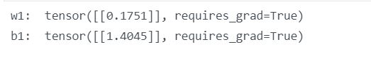
Let us check the optimized value for W1 and b1:

print ('w1: ', w1)
print ('b1: ', b1)

Getting the prediction values using the weights in the linear equation.

predicted_in_tensor = x_train_tensor.mm(w1).clamp(min=0).add(b1)

Visualizing the Prediction and Actual values

plt.figure(figsize=(8, 8))
plt.scatter(x_train, y_train, c='green', s=200, label='Original data')
plt.plot(x_train, predicted, label = 'Fitted line')
plt.legend()
plt.show()

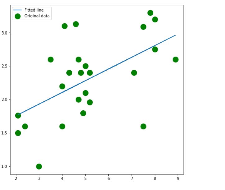
So, here we have it. A simple linear model, built and trained using PyTorch. There are various ways to build a simple linear model, but through this tutorial, you got to understand and get familiar with some of the critical functions in PyTorch to create a neural network. This time it was a neuron, but these same things can be expanded into something more robust and optimal particularly by adding activation function or working with multiple neurons or both. You can easily form them into a full-fledged deep neural network. I suggest you try and make multiple neural structures and deepen your understanding using PyTorch.

I hope, you find this article useful and if not already, get started with PyTorch and build interesting models. Thank you.

Gargeya Sharma

B.Tech 4th Year Student
Specialized in Deep Learning and Data Science

For getting more info check out my Github Homepage

LinkedIn

GitHub

Gargeya Sharma 04 Apr 2023