Implementation of Gaussian Naive Bayes in Python Sklearn
This article was published as a part of the Data Science Blogathon.
Introduction
Consider the following scenario: you are a product manager who wants to categorize customer feedback into two categories: favorable and unfavorable. Or As a loan manager, do you want to know which loan applications are safe to lend to and which ones are risky? As a healthcare analyst, you want to be able to forecast which patients are likely to develop diabetic complications. All of the instances have the same kind of challenge when it comes to categorizing reviews, loan applications, and patients, among other things.
Naive Bayes is the easiest and rapid classification method available, and it is well suited for dealing with enormous amounts of information. In several applications such as spam filtering, text classification, sentiment analysis, and recommender systems, the Naive Bayes classifier has shown to be effective. It makes predictions about unknown classes using the Bayes theory of probability.
We will go through the Naive Bayes classification course in Python Sklearn in this article. We will explain what is Naive Bayes algorithm is and continue to view an end-to-end example of implementing the Gaussian Naive Bayes classifier in Sklearn using a dataset.
Table of contents
What is Naive Bayes Algorithm?
Naive Bayes is a basic but effective probabilistic classification model in machine learning that draws influence from Bayes Theorem.
Bayes theorem is a formula that offers a conditional probability of an event A taking happening given another event B has previously happened. Its mathematical formula is as follows: –
.png)
Where
- A and B are two events
- P(A|B) is the probability of event A provided event B has already happened.
- P(B|A) is the probability of event B provided event A has already happened.
- P(A) is the independent probability of A
- P(B) is the independent probability of B
Now, this Bayes theorem can be used to generate the following classification model –
.png)
Where
- X = x1,x2,x3,.. xN аre list оf indeрendent рrediсtоrs
- y is the class label
- P(y|X) is the probability of label y given the predictors X
The above equation may be extended as follows:
.png)
Characteristics of Naive Bayes Classifier
- The Naive Bayes method makes the assumption that the predictors contribute equally and independently to selecting the output class.
- Although the Naive Bayes model’s assumption that all predictors are independent of one another is unfeasible in real-world circumstances, this assumption produces a satisfactory outcome in the majority of instances.
- Naive Bayes is often used for text categorization since the dimensionality of the data is frequently rather large.
Types of Naive Bayes Classifiers
Naive Bayes Classifiers are classified into three categories —
i) Gaussian Naive Bayes
This classifier is employed when the predictor values are continuous and are expected to follow a Gaussian distribution.
ii) Bernoulli Naive Bayes
When the predictors are boolean in nature and are supposed to follow the Bernoulli distribution, this classifier is utilized.
iii) Multinomial Naive Bayes
This classifier makes use of a multinomial distribution and is often used to solve issues involving document or text classification.
Example of a Gaussian Naive Bayes Classifier in Python Sklearn
We will walk you through an end-to-end demonstration of the Gaussian Naive Bayes classifier in Python Sklearn using a cancer dataset in this part. For our example, we’ll use SKlearn’s Gaussian Naive Bayes function, i.e. GaussianNB().
Step-1: Loading Initial Libraries
We’ll begin by loading some basic libraries that will be used to import and view the dataset.
import numpy as np
import pandas as pd
import matplotlib.pyplot as plt
Step-2: Importing Dataset
Now, we’ll submit the cancer detection dataset from Kaggle that we used to do our Naive Bayes classification.
dataset = pd.read_csv("datasets/cancer.csv")
Step-3: Exploring Dataset
Let’s take a quick look at the dataset using the head() method.
Python Code:
Following that, we’ll analyze the columns included inside the dataset using the info() method.
Input:
dataset.info()
Output:
RangeIndex: 569 entries, 0 to 568
Data columns (total 33 columns):
 #   Column                   Non-Null Count  Dtype
---  ------                   --------------  -----
 0   id                       569 non-null    int64
 1   diagnosis                569 non-null    object
 2   radius_mean              569 non-null    float64
 3   texture_mean             569 non-null    float64
 4   perimeter_mean           569 non-null    float64
 5   area_mean                569 non-null    float64
 6   smoothness_mean          569 non-null    float64
 7   compactness_mean         569 non-null    float64
 8   concavity_mean           569 non-null    float64
 9   concave points_mean      569 non-null    float64
 10  symmetry_mean            569 non-null    float64
 11  fractal_dimension_mean   569 non-null    float64
 12  radius_se                569 non-null    float64
 13  texture_se               569 non-null    float64
 14  perimeter_se             569 non-null    float64
 15  area_se                  569 non-null    float64
 16  smoothness_se            569 non-null    float64
 17  compactness_se           569 non-null    float64
 18  concavity_se             569 non-null    float64
 19  concave points_se        569 non-null    float64
 20  symmetry_se              569 non-null    float64
 21  fractal_dimension_se     569 non-null    float64
 22  radius_worst             569 non-null    float64
 23  texture_worst            569 non-null    float64
 24  perimeter_worst          569 non-null    float64
 25  area_worst               569 non-null    float64
 26  smoothness_worst         569 non-null    float64
 27  compactness_worst        569 non-null    float64
 28  concavity_worst          569 non-null    float64
 29  concave points_worst     569 non-null    float64
 30  symmetry_worst           569 non-null    float64
 31  fractal_dimension_worst  569 non-null    float64
 32  Unnamed: 32              0 non-null      float64
dtypes: float64(31), int64(1), object(1)
memory usage: 146.8+ KB
We can see from the information above that the id and unnamed:32 columns are not relevant, so we can eliminate them.
Input:
dataset = dataset.drop(["id"], axis = 1)
Input:
dataset = dataset.drop(["Unnamed: 32"], axis = 1)
Step-4: Visualizing Dataset
Malignant Tumor Dataframe
Input:
M = dataset[dataset.diagnosis == "M"]
Benign Tumor Dataframe
Input:
B = dataset[dataset.diagnosis == "B"]
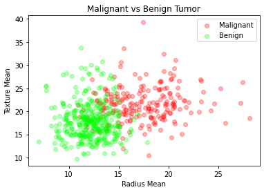
We shall now examine malignant and benign tumors by examining their average radius and texture.
Input:
plt.title("Malignant vs Benign Tumor")
plt.xlabel("Radius Mean")
plt.ylabel("Texture Mean")
plt.scatter(M.radius_mean, M.texture_mean, color = "red", label = "Malignant", alpha = 0.3)
plt.scatter(B.radius_mean, B.texture_mean, color = "lime", label = "Benign", alpha = 0.3)
plt.legend()
plt.show()
Output:
Step-5: Preprocessing
Now, malignant tumors will be assigned a value of ‘1’ and benign tumors will be assigned a value of ‘0’.
Input:
dаtаset.diаgnоsis = [1 if i== "M" else 0 fоr i in dаtаset.diаgnоsis]
We now divide our dataframe into x and y components. The x variable includes all independent predictor factors, whereas the y variable provides the diagnostic prediction.
Input:
x = dataset.drop(["diagnosis"], axis = 1)
y = dataset.diagnosis.values
Step-6: Data Normalization
To maximize the model’s efficiency, it’s always a good idea to normalize the data to a common scale.
Input:
# Normalization:
x = (x - nр.min(x)) / (nр.mаx(x) - nр.min(x))
Step-7: Test Train Split
After that, we’ll use the train test split module from the sklearn package to divide the dataset into training and testing sections.
Input:
from sklearn.model_selection import train_test_split
x_train, x_test, y_train, y_test = train_test_split(x, y, test_size = 0.3, random_state = 42)
Step-8: Sklearn Gaussian Naive Bayes Model
Now we’ll import and instantiate the Gaussian Naive Bayes module from SKlearn GaussianNB. To fit the model, we may pass x_train and y_train.
Input:
from sklearn.naive_bayes import GaussianNB
nb = GaussianNB()
nb.fit(x_train, y_train)
Output:
GaussianNB()
Step-9: Accuracy
The following accuracy score reflects how successfully our Sklearn Gaussian Naive Bayes model predicted cancer using the test data.
Input:
print("Naive Bayes score: ",nb.score(x_test, y_test))
Output:
Naive Bayes score: 0.935672514619883
Frequently Asked Questions
A. To use the Naive Bayes classifier in Python using scikit-learn (sklearn), follow these steps:
1. Import the necessary libraries: from sklearn.naive_bayes import GaussianNB
2. Create an instance of the Naive Bayes classifier: classifier = GaussianNB()
3. Fit the classifier to your training data: classifier.fit(X_train, y_train)
4. Predict the target values for your test data: y_pred = classifier.predict(X_test)
5. Evaluate the performance of the classifier: accuracy = classifier.score(X_test, y_test)
A. No, Naive Bayes is not considered a lazy classifier. The term “lazy classifier” typically refers to algorithms that delay the learning process until the time of prediction. These algorithms store the training instances and use them directly during the prediction phase.
In contrast, Naive Bayes is an example of an eager or “generative” classifier. It learns a probabilistic model based on the training data during the training phase, and this model is then used to make predictions on new, unseen instances without requiring the original training data at prediction time.
Conclusion
Naive Bayes is the simplest and most powerful algorithm. Despite recent major breakthroughs in Machine Learning, it has shown its utility. It’s been used in applications ranging from text analytics to recommendation systems.
After explaining Naive Bayes and demonstrating an end-to-end implementation of Gaussian Naive Bayes in Sklearn using the Cancer dataset, we have reached the finish of this article. Thank you for reading it! I really hope you found this brief introductory training to be informative.
I hope you like the content. If you’d like to contact me, you may do so via:
or you can send me an email if you have any further queries.
The media shown in this article is not owned by Analytics Vidhya and are used at the Author’s discretion
Currently, I Am pursuing my Bachelors of Technology( B.Tech) from Vellore Institute of Technology. I am very enthusiastic about programming and its real applications including software development, machine learning and data science.


