During the Machine Learning model building, the Regularization Techniques is an unavoidable and important step to improve the model prediction and reduce errors. This is also called the Shrinkage method. Which we use to add the penalty term to control the complex model to avoid overfitting by reducing the variance.
Let’s discuss the available methods, implementation, and benefits of those in detail here.
The too many parameters/attributes/features along with data and those permutations and combinations of attributes would be sufficient, to capture the possible relationship within dependent and independent variables.
To understand the relationship between the target and available independent variables with several permutations and combinations. For this exercise certainly, we need adequate data in terms of records or datasets for our analysis, hope you are aware of that.
If you have fewer data with huge attributes the depth vs breadth analysis there might lead to that not all possible permutations and combinations among the dependent and independent variables. So those missing values force good or bad to your model. Of course, we can call out this circumstance as Curse of Dimensionality. Here we are looking for these aspects from data along with parameters/attributes/features.
Curse of Dimensionality is not directly mean that too many dimensions, this is the lack of possible permutation and combination.
In another way round the missing data and gap generates empty space, so we couldn’t connect the dots and create the perfect model. It means that the algorithm cannot understand the data and spread across with given space or empty, with multi-dimensional mode and meets with kind of relationship between dependent and independent variables and predicting the future data. If you try to visualize this, it would be really complex format and difficult to follow.
During the training, you will get the above-said observation, but during the testing, the new and not exposed data combination to model’s accuracy will jump across and it suffers from error, because of variance [variance error] and not fit for production move and risk for prediction.
Due to the too many Dimensions with too few data, the algorithm would build the best fit with peaks and deep-down dells in the observation along with the high magnitude of coefficient its leads to overfitting and is not suitable for production. [drastic fluctuation in surface inclination]
To understand or implement these techniques, we should understand the cost function of your linear models.
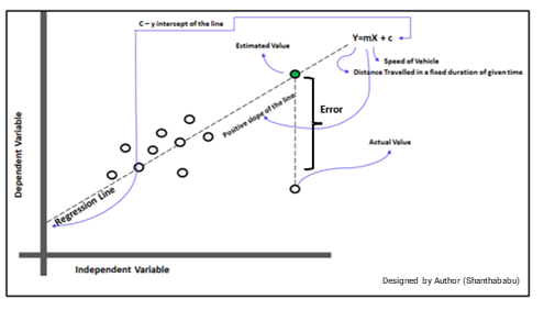
Understanding the Regression Graph
The below graph represents the entire parameters existing in the LR model and is very self-explanatory.
Significance Of Cost Function
Cost function/Error function: Takes slope-intercept (m and c) values and returns the error value/cost value. It shows the error between predicted outcomes is compared with the actual outcomes. It explains how your model is inaccurate in its prediction.
It is used to estimate how badly models are performing for the given dataset and its dimensions.
Why is cost function important in machine learning? Yes, the cost function helps us reach the optimal solution, So how can we do this. will see all possible methods and simple steps using Python libraries.
This function helps us to a figure-out best straight line by minimizing the error
The best fit line is that line where the sum of squared errors around the line is minimized
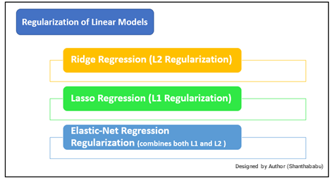
Regularization Techniques
Let’s discuss the available Regularization techniques and followed by the implementation
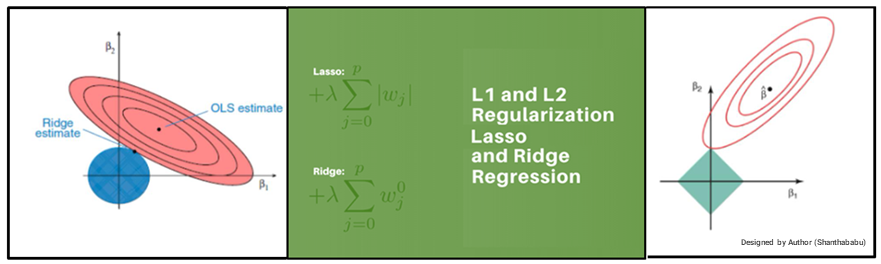
1. Ridge Regression (L2 Regularization):
Basically here, we’re going to minimize the sum of squared errors and sum of the squared coefficients (β). In the background,
the coefficients (β) with a large magnitude will generate the graph peak and
deep slope, to suppress this we’re using the lambda (λ) use to be called a
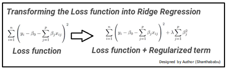
Penalty Factor and help us to get a smooth surface instead of an irregular-graph. Ridge Regression is used to push the coefficients(β) value nearing zero in terms of magnitude. This is L2 regularization, since its adding a penalty-equivalent to theSquare-of-the Magnitude of coefficients.
Ridge Regression = Loss function + Regularized term
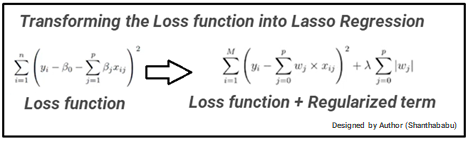
2. Lasso Regression (L1 Regularization):
This is very similar to Ridge Regression, with little difference in Penalty Factor that coefficient is magnitude instead of squared. In which there are possibilities of many coefficients becoming zero, so that corresponding attribute/features become zero and dropped from the list, this ultimately reduces the dimensions and supports for dimensionality reduction. So which deciding that those attributes/features are not suitable as predators for predicting target value. This is L1 regularization, because of adding the Absolute-Value as penalty-equivalent to the magnitude of coefficients.
Lasso Regression = Loss function + Regularized term
3. Characteristics of Lambda
λ = 0
λ => Minimal
λ =>High
Lambda or Penalty Factor (λ)
No impact on coefficients(β) and model would be Overfit. Not suitable
for Production
Generalised model and acceptable accuracy and eligible for Test and
Train. Fit for Production
Very high impact on coefficients (β) and leading to underfit. Ultimately
not fit for Production.
Remember one thing that the Ridge never make coefficients into zero, Lasso will do. So, you can use the second one for feature selection.
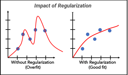
Impact of Regularization
The below graphical representation clearly indicates the best fitment.
4. Elastic-Net Regression Regularization:
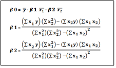
Even though Python provides excellent libraries, we should understand the mathematics behind this. Here is the detailed derivation for your reference.
Ridge: α=0
Lasso: α=1
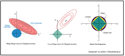
5. Pictorial representation of Regularization Techniques
Mathematical approach for L1 and L2
Even though Python provides excellent libraries and straightforward coding, we should understand the mathematics behind this. Here is the detailed derivation for your reference.
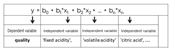
Let’s have below multi-linear regression dataset and its equation
As we know Multi-Linear-Regression
y=β0+ β1 x1+ β2 x2+………………+ βn xn —————–1
yi= β0+ Σ βi xi —————–2
Σ yi– β0– Σ βi xi
Cost/Loss function: Σ{ yi– β0– Σ βi xij}2—————–3
Regularized term: λΣ βi2—————-4
Ridge Regression = Loss function + Regularized term—————–5
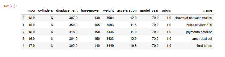
Let’s take Automobile – Predictive Analysis and apply the L1 and L2 and how it helps model score.
Objective: Predicting the Mileage/Miles Per Gallon (mpg) of a car using given features of the car.
print("*************************")

print("Import required libraries")

print("*************************")

%matplotlib inline

import numpy as np

import pandas as pd

import seaborn as sns

import matplotlib.pyplot as plt

from sklearn.linear_model import LinearRegression

from sklearn.linear_model import Ridge

from sklearn.linear_model import Lasso

from sklearn.metrics import r2_score
Output
Python Code:
*************************
 Using auto-mpg dataset
*************************
EDA: Will do little EDA (Exploratory Data Analysis), to understand the dataset
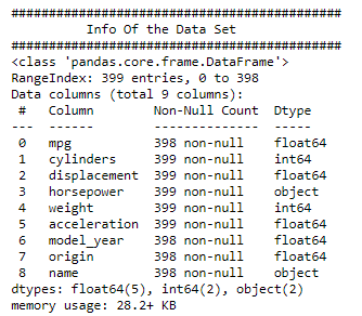
print("############################################")
print("          Info Of the Data Set")
print("############################################")
df_cars.info()
Observation:
1. we could see that the features and its data type, along with Null constraints.
2. Horsepower and name features are objects in the given data set. have to take care of during the modelling.
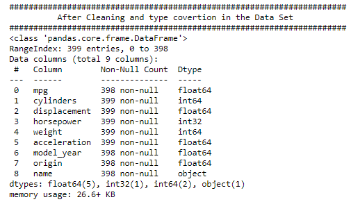
Data Cleaning/Wrangling:
Is the process of cleaning and consolidating the complex data sets for easy access and analysis.
Action:
replace(‘?’,’NaN’)
Converting “horsepower” Object type into int
df_cars.horsepower = df_cars.horsepower.str.replace('?','NaN').astype(float)
df_cars.horsepower.fillna(df_cars.horsepower.mean(),inplace=True)
df_cars.horsepower = df_cars.horsepower.astype(int)
print("######################################################################")
print("          After Cleaning and type covertion in the Data Set")
print("######################################################################")
df_cars.info()
Observation:
1. We could see that the features/column/fields and its data type, along with Null count
2. horsepower is now int type and name still as an object type in the given data set, since this column not going to support either way as preditors.
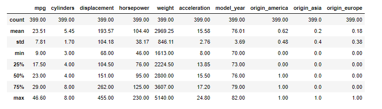
# Statistics of the data
display(df_cars.describe().round(2))
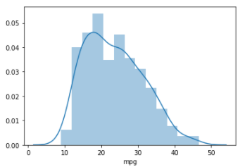
# Skewness and kurtosis
print("Skewness: %f" %df_cars['mpg'].skew())
print("Kurtosis: %f" %df_cars['mpg'].kurt())
Output: Look at the curve and how it is distributed across and see the same.
regression_model = LinearRegression()
regression_model.fit(X_train, y_train)
for idcoff, columnname in enumerate(X_train.columns):
    print("The coefficient for {} is {}".format(columnname, regression_model.coef_[0][idcoff]))
Output: Try to understand the coefficient (βi)
The coefficient for cylinders is -0.08627732236942003
The coefficient for displacement is 0.385244857729236
The coefficient for horsepower is -0.10297215401481062
The coefficient for weight is -0.7987498466220165
The coefficient for acceleration is 0.023089636890550748
The coefficient for model_year is 0.3962256595226441
The coefficient for origin_america is 0.3761300367522465
The coefficient for origin_asia is 0.43102736614202025
The coefficient for origin_europe is 0.4412719522838424
intercept = regression_model.intercept_[0]
print("The intercept for our model is {}".format(intercept))
Output
The intercept for our model is 0.015545728908811594
Scores (LR)
Output: Compare with LR model coefficient and RIDGE, Here you could see that the few coefficients and zeroed (0) and during the fitment, they are excluded from the feature list.
Certainly, there is an impact on the model due to the Regularization L2 and L1.
Compare L2 and L1 Regularization
Hope after seeing the code level implementation, you could able to relate the importance of regularization techniques and their influence on the model improvements. As a final touch let’s compare the L1 & L2.
Ridge Regression (L2)
Lasso Regression(L1)
Quite accurate and keep all features
More Accurate than Ridge
λ ==> Sum of the squares of coefficient
λ ==> Sum of the absolute of coefficient.
The coefficient can be not to zeroed, but rounded
The coefficient can be zeroed
Variable selection and keeping all variables
Model selection by dropping coefficient
Differentiable and leading for gradient descent calculation
Not differentiable
Model fitment justification during training and testing
Model is doing strongly at training set and poorly in test set means we’re at OVERFIT
Model is doing poor at both (Training and Testing) means we’re at UNDERFIT
Model is doing better and considers ways in both (Training and Test), means we’re at the RIGHT FIT
Conclusion
I hope, what we have discussed so for, would really help you all how and why regularization techniques are important and inescapable while building a model. Thanks for your valuable time in reading this article. Will get back to you with some interesting topics. Until then Bye! Cheers! Shanthababu.
The media shown in this article is not owned by Analytics Vidhya and are used at the Author’s discretion
A verification link has been sent to your email id
If you have not recieved the link please goto
Sign Up page again
Loading...
Please enter the OTP that is sent to your registered email id
Loading...
Please enter the OTP that is sent to your email id
Loading...
Please enter your registered email id
This email id is not registered with us. Please enter your registered email id.
Don't have an account yet?Register here
Loading...
Please enter the OTP that is sent your registered email id
Loading...
Please create the new password here
We use cookies on Analytics Vidhya websites to deliver our services, analyze web traffic, and improve your experience on the site. By using Analytics Vidhya, you agree to our Privacy Policy and Terms of Use.Accept
Privacy & Cookies Policy
Privacy Overview
This website uses cookies to improve your experience while you navigate through the website. Out of these, the cookies that are categorized as necessary are stored on your browser as they are essential for the working of basic functionalities of the website. We also use third-party cookies that help us analyze and understand how you use this website. These cookies will be stored in your browser only with your consent. You also have the option to opt-out of these cookies. But opting out of some of these cookies may affect your browsing experience.
Necessary cookies are absolutely essential for the website to function properly. This category only includes cookies that ensures basic functionalities and security features of the website. These cookies do not store any personal information.
Any cookies that may not be particularly necessary for the website to function and is used specifically to collect user personal data via analytics, ads, other embedded contents are termed as non-necessary cookies. It is mandatory to procure user consent prior to running these cookies on your website.


Hi, It is really a very interesting and important article for me. Thanks a lot for sharing. by PSK