A Brief Introduction To Yandex-Catboost Regressor

This article was published as a part of the Data Science Blogathon

Overview

CATBOOST is an open-source machine learning library developed by a Russian search engine giant Yandex. One of the prominent aspects of catboost is its ability to handle missing data and categorical data without encoding but will get to that later. It makes feature engineering tasks easier and in some cases extinct. As the name suggests it’s a boosting algorithm, building trees sequentially and reducing error in each iteration. Though catboost isn’t as popular(Google trends show the popularity of catboost vs xgboost vs lightgbm) as XGBoost, it’s a powerful library and a good one to explore. In addition to regression and classification tasks, it can also be used for forecasting as well as recommendation systems.

trends.embed.renderExploreWidget(“TIMESERIES”, {“comparisonItem”:[{“keyword”:”catboost”,”geo”:”IN”,”time”:”today 12-m”},{“keyword”:”/g/11clwl3wbz”,”geo”:”IN”,”time”:”today 12-m”},{“keyword”:”/g/11hh69zqkh”,”geo”:”IN”,”time”:”today 12-m”}],”category”:0,”property”:””}, {“exploreQuery”:”geo=IN&q=catboost,%2Fg%2F11clwl3wbz,%2Fg%2F11hh69zqkh&date=today 12-m,today 12-m,today 12-m”,”guestPath”:”https://trends.google.com:443/trends/embed/”});

Table of contents

1. Problem Statement
2. Read and describe data
3. Basic data exploration
4. Build baseline model
5. Better than baseline model version 001
6. Better than baseline model version 002
7. Common CATBOOST parameters
8. Common CATBOOST errors
9. Predict and save results

Problem Statement

India has quite a lot of credit card providers majorly banks, who provide credit based on Credit score/CIBIL score. Alternatively, there are credit card start-ups like Slice or OneCard, etc. which do not exclusively rely on credit scores. This particular dataset has various customer and property dimensions and metrics. Given the customer, characteristics predict the max loan amount that can be sanctioned for a particular property.

https://www.godigit.com/finance/credit-score/what-is-a-good-credit-score

Read and describe data

Data for this tutorial can be downloaded using this link. A custom utils function is used to load, explore and clean data. The same can be downloaded from this link.

## utils functions
%run extras/lab_utils_cls.ipynb

test_file_loc = "https://raw.githubusercontent.com/chrisdmell/DataScience/master/data_dump/01_cipla_ds_challenge/test.csv"
train_file_loc = "https://raw.githubusercontent.com/chrisdmell/DataScience/master/data_dump/01_cipla_ds_challenge/train.csv"

df_insurance = Utils.load_data(test_file_loc)
df_insurance_train = Utils.load_data(train_file_loc)

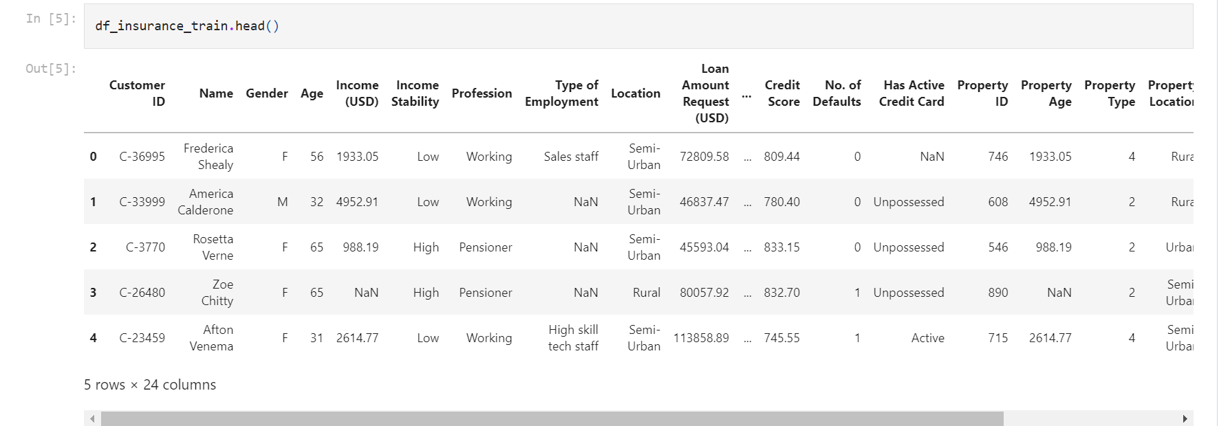
Description of the columns in the dataset –

As the dataset has missing values, this function provides % missing values for each column

    @staticmethod
    def missing_percentage(df_insurance_train, other_dict = {}):
        '''
        input is a dataframe
        returns : the percentage of missing values
        '''
        missing_df = df_insurance_train.isnull().sum().reset_index()
        missing_df["total"] = len(df_insurance_train)
        missing_df.columns = ["features", "null_count", "total"]
        missing_df["missing_percent"] = round(missing_df["null_count"]/missing_df.total*100, 2)
        missing_df.sort_values("missing_percent", ascending = False, inplace = True)
        print(missing_df.to_markdown())
        return missing_df

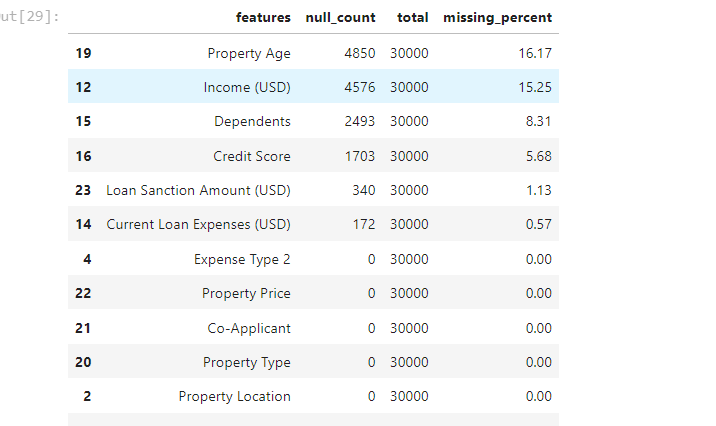
Only 6 columns have NULL values, and the rest of the columns can be used without any data cleaning or manipulation. Usually, more than 20% of missing values would render the variable ineffective, the best course of action is to either drop the variable or impute.

Basic data exploration

Building hypotheses and validating them is a key aspect of solving a data science problem. For this particular dataset few questions that can be asked are:

Correlation plot

import seaborn as sns
f, ax = plt.subplots(figsize=(10, 8))
corr = df_insurance_train[hist_cols].corr()
sns.heatmap(corr, mask=np.zeros_like(corr, dtype=np.bool), cmap=sns.diverging_palette(240, 10, as_cmap=True),
            square=True, ax=ax)

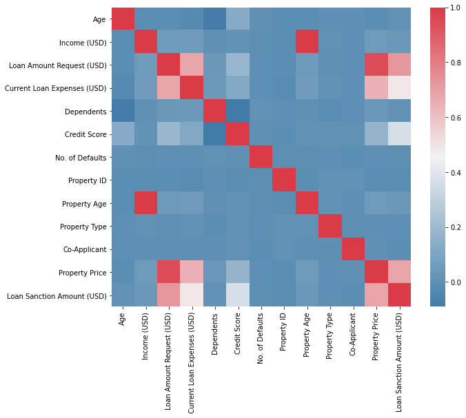
There are clear correlations between –

1. Current loan expenses and the loan amount requested.
2. Property age and income.
3. Property price and the loan amount requested.
4. Property price and current loan expenses

How to determine which variables to ignore and which ones to keep? The feature importance attribute of catboost will be of help in making this decision. The variables with the least feature importance can be ignored.

Plot Categorical Variables

  @staticmethod
    def plot_categorical_bar(df_insurance_train):
        '''
        Input data frame -
        Bar plot for all columns which are not float or int
        Keep top ten sorted high to low - this can be a variable
        '''
        df = dict(df_insurance_train.dtypes)
        hist_cols = [key for key in df.keys() if (df[key] == "int64" or df[key] == "float64")]
        a = list(df_insurance_train.columns)
        b = hist_cols
        categorical_columns = list(set(a)-set(b))
        for col in categorical_columns:
            print(col)
            ## the output of value_counts is pandas series and we can directly pass it to pandas DataFrame method to get a df
            ## value_count gives multi index so reset
            v_cont = pd.DataFrame(df_insurance_train[[col]].value_counts().reset_index())
            ## assign common column names
            v_cont.columns = ["feature", "count"]
            ## Sort descning and limit to top 10
            v_cont.sort_values("count", axis = 0, ascending = False, inplace = True)
            v_cont = v_cont[0:10]
            ax = sns.barplot(x="feature", y="count", data=v_cont)
            ##reset index as iterrows() will iterate over index
            v_cont.reset_index(inplace = True)
            for index, row in v_cont.iterrows():
                ax.text(row.name,row["count"], round(row["count"],2), color='black', ha="center")
            ## dropping pandas bar plot
            #ax = v_cont.plot.bar()
            plt.xticks(rotation = 45)  ## rotate x lables by 45 degrees
            plt.title(col)
            plt.show()
        #     v_cont.index = v_cont.feature
        #     for index, value in enumerate(v_cont.count):
        #         plt.text(index,value, str(value))

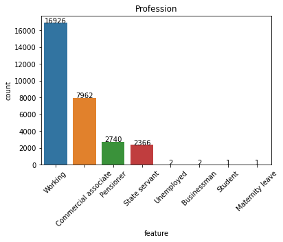
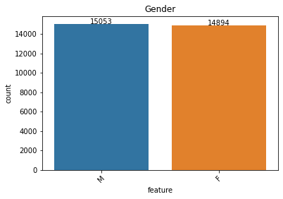
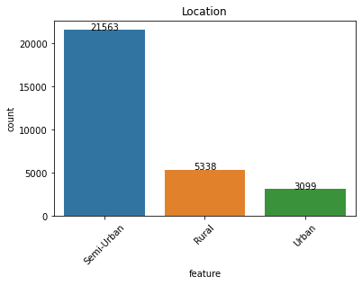
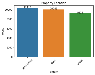
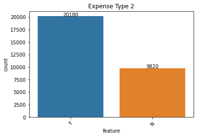
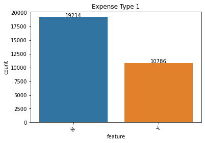
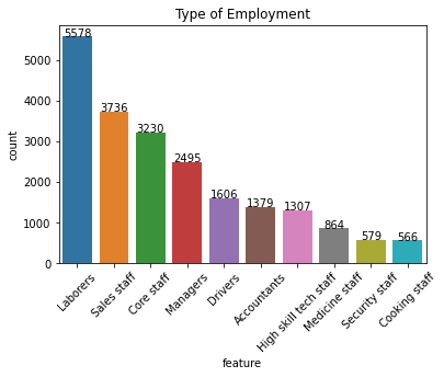
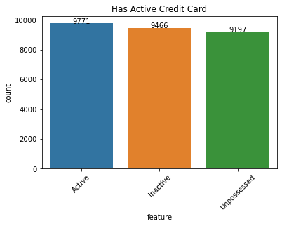
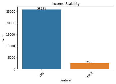
Salient points:

1. A nearly equal amount of male and female applicants.
2. Labourer’s and sales staff dominate the employment type.
3. Even though properties are located equally amongst rural/semi-urban/urban areas, the majority of the applicants are semi-urban.
4. Expense type shows some variation and low-income stability individuals seem to dominate these applications.

Plot Numeric Variables

@staticmethod
    def hist_flt_int(dataset):
        '''
        From the df.dtypes, which is pandas series, we convert to dict then get use list comprehension to get the 
        column name with int and float
        input - dataframe
        output - histogram of int and floats
        '''
        ## TODO : Image size config
        df = dict(dataset.dtypes)
        hist_cols = [key for key in df.keys() if (df[key] == "int64" or df[key] == "float64")]
        fig = plt.figure(figsize = (15,20))
        ax = fig.gca()
        return dataset[hist_cols].hist(ax = ax)

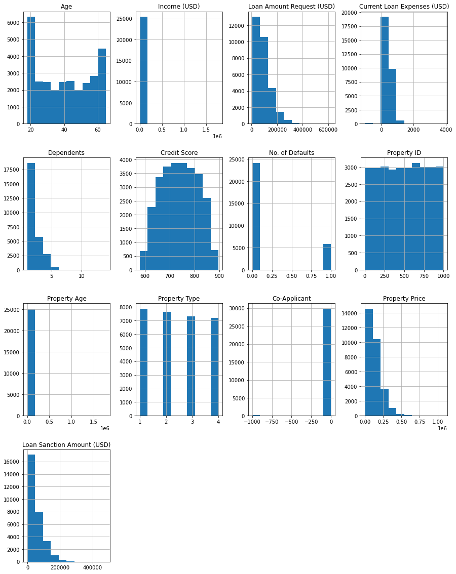
Salient points:

1. Age – The majority of the applicants are young @20.
2. The loan amount sanctioned is right-skewed, the majority of loan applications are small scale.
3. A large # of applicants have less than 2 dependents.
4. Credit scores are normally distributed.
5. The majority of the applicants haven’t defaulted before.
6. Income and property age needs to be scaled or transformed to be able to contribute to the model.
7. Property price and loan amount sanctioned is right-skewed.

It would help to transform right-skewed data to normal distribution.

Build baseline model:

The idea of the baseline model is to build a simple model without heavy data cleaning, imputation, and manipulation. To build a basic model to get a sense of the complexity of the problem.

In catboost, the categorical columns need not be encoded, instead, a list of categorical column names needs to be passed a parameter. The catboost regressor class used in the code can be found here.

Install CATBOOST:

!pip install catboost

Non-Null columns are used to build the baseline model. Loss function – RMSE (root mean squared error ) is used and the model is trained for 100 iterations. One aspect to keep in mind is RMSE is sensitive to outliers, so it’s imperative to treat outliers while building more working models.

columns_to_keep = [ 'Gender', 'Age', 'Income (USD)',
       'Income Stability', 'Profession', 'Type of Employment', 'Location',
       'Loan Amount Request (USD)', 'Current Loan Expenses (USD)',
       'Expense Type 1', 'Expense Type 2', 'Dependents', 'Credit Score',
       'No. of Defaults', 'Has Active Credit Card', 
       'Property Age', 'Property Type', 'Property Location', 'Co-Applicant',
       'Property Price', 'Loan Sanction Amount (USD)']
var_dict = {}
var_dict["independant"] = ['Gender','Age', 'Income (USD)',
       'Income Stability', 'Profession', 'Type of Employment', 'Location',
       'Loan Amount Request (USD)', 'Current Loan Expenses (USD)',
       'Expense Type 1', 'Expense Type 2', 'Dependents', 'Credit Score',
       'No. of Defaults', 'Has Active Credit Card', 
       'Property Age', 'Property Type', 'Property Location', 'Co-Applicant',
       'Property Price']
cat_features = ['Gender',
       'Income Stability', 'Profession', 'Type of Employment', 'Location',
       'Expense Type 1', 'Expense Type 2', 'Dependents',
       'No. of Defaults', 'Has Active Credit Card', 
       'Property Type', 'Property Location', 'Co-Applicant']
var_dict["dependant"]   = ["Loan Sanction Amount (USD)"]
features_to_keep = df_insurance_train[columns_to_keep]
features_to_keep[cat_features] = features_to_keep[cat_features].astype(str)
features_to_keep.dropna(inplace =  True)  ## this cannot be done in test becauase we need all the 20K samples
params = {"cat_features": cat_features, "loss_function": "RMSE", "iterations" : 100}
cat_model = catboost_regressor.new_instance(params)
rf_model_output = cat_model.model_run(features_to_keep, var_dict, )

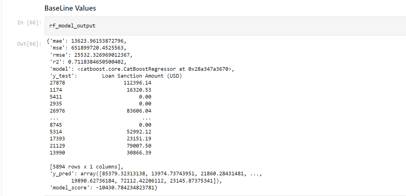
The evaluation metrics are as follows RMSE of 25532 and R² of 71%. R² score shows how well the model fits the data. The minimum bar has been set, any model further developed has to be better than this minimum bar. A baseline model helps allay the fear and nervousness of building a model.

Better than baseline model version 001

Few columns have NULL values and special characters, what can be done to clean this dataset? Note – Never use one-hot encoding while using Catboost, the model takes a long time to train and the will be performance degradation.

Fill null values in the dependent variables with 0

df_insurance_train["Loan Sanction Amount (USD)"].fillna(0, inplace = True)

For other numeric columns fill NULL with mean values of the columns

    @staticmethod
    def num_col_mean_impute(df_insurance_train, num_impute_dict, other_dict = {}):
        '''
        inputs:
        df_insurance_train - train dataframe with 
        num_impute_dict - 
        num_impute_dict = {"Property Age" : ["Profession", "mean"], "Income (USD)":["Profession",  "mean"],
                   "Dependents":["", "mode"] , "Credit Score":["Has Active Credit Card", "mean"],
                  "Loan Sanction Amount (USD)":["", 0], "Current Loan Expenses (USD)":["Profession", "mean"]}
        The idea is to DO MORE, rn doing the minimum,
        {"Property Age" : ["Profession", "mean"]} - The idea is, impute proterty age with mean property age of profession columns. 
        Business ideas, same profession guys look for similar property age. 
        A godown guy will look for older buildings, but a technie will look for new homes. 
        '''
        impute_df = pd.DataFrame(num_impute_dict)
        ## helps to pretty print in jupyter we use to_markdown()
        print(num_impute_dict)
#         print(impute_df)
        ## loop over the df
        for cols in impute_df.columns:
            print(cols)
            x = impute_df[[cols]]
#             print(x.columns[0]) 
            ## fillna with column mean.
            df_insurance_train[cols].fillna(value= df_insurance_train[cols].mean(), inplace=True)
        DataClean.missing_percentage(df_insurance_train)
        return df_insurance_train

For categorical values, replace null with a categorical value such as missing_value. NULL doesn’t explicitly mean the values are missing due to some error, it could also mean the values are missing on purpose. For example – Gender, if a person doesn’t relate to either of the more common genders, it could be left blank or someone might not want to disclose the type of employment, all these are genuine real-world issues.

    @staticmethod
    def null_to_missing_cat(df_insurance_train, other_dict = {}):
        '''
        Input data frame with np.nan values and pandas NULL
        fillna() misses out np.nan
        NAN and NONE are interchangable in pandas
        All null values are convereted to a class called missing_value
        Output : pandas df with same shape
        '''
        df = dict(df_insurance_train.dtypes)
        hist_cols = [key for key in df.keys() if (df[key] == "int64" or df[key] == "float64")]
        a = list(df_insurance_train.columns)
        b = hist_cols
        categorical_columns = list(set(a)-set(b))
        df_numeric = df_insurance_train[hist_cols]
        ## replace null values
        df_insurance_train[categorical_columns].fillna('missing_value', inplace=True)
        df_categorical = df_insurance_train[categorical_columns].replace(np.nan, 'missing_value', regex=True) # All data frame
        df_insurance_train =  pd.concat([df_categorical.reset_index(drop=True), df_numeric], axis=1)
        DataClean.missing_percentage(df_insurance_train)
        return(df_insurance_train)

We build the model again, after a few data manipulation.

params = {"cat_features": cat_features, "loss_function": "RMSE", "iterations" : 100}
cat_model = catboost_regressor.new_instance(params)
cat_model_output_002 = cat_model.model_run(features_to_keep, var_dict, )

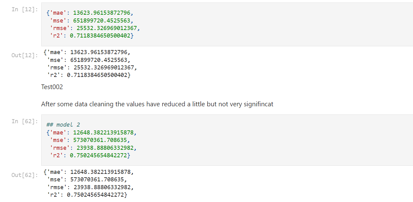
It is clear that the imputations and manipulation have had a positive impact on the model. The RMSE reduced to 23938 and R² increased to 75%.

6. Better than baseline model version 002:

Now that a better model than a baseline is built, it’s time to refine the model and improve its accuracy.

One aspect that can be tried is to log transform the dependent variable np.log(df[label]+1). This will improve the model performance drastically.

It’s also cumbersome to keep track of all the models and it’s parameters, the more models the more parameter, and along with it comes the task to log everything. An open-source library called MLFLOW makes this task easier. This Analytics Vidhya article sheds light on how to use MLFLOW to log machine learning experiments.

CATBOOST also supports SHAP plots to explore the effects of features on target variables. Feature importance can also be plotted to understand what features can be left out.

Common CATBOOST parameter

While using any library for the first time, there are bound to be errors, some of the common errors are listed below.

params = {"cat_features": cat_features, "loss_function": "RMSE", 
          "random_seed" : 42,
#           "iterations" : 100, 
          "verbose":0,
         'learning_rate': 0.1,
#          'depth': 8,   ##depth of the trees
         'l2_leaf_reg': 40, 
         "max_depth" : 10,  #max depth /depth of 10 makes sense 
         "model_size_reg" : 5,
         "n_estimators": 1000,
         "random_strength": 0.4,  #We use randomness when scoring the splits. Every split gets a score and then we add some randomness to it, this helps to reduce overfitting.
#          "bootstrap_type " :"Bayesian",
          "bagging_temperature": 2,    # 0 to +infty  / Only with Bayesian bootstraping
          "eval_metric" : "MSLE" , #The metric used for overfitting detection 
          "grow_policy": "Lossguide" , # The tree growing policy. Defines how to perform greedy tree construction.
        "min_data_in_leaf" :  10,  # The minimum number of training samples in a leaf. CatBoost does not search for new splits in leaves with samples count less than the specified value.
                              # Can be used only with the Lossguide and Depthwise growing policies.
        "one_hot_max_size": 4, # Use one-hot encoding for all categorical features with a number of different values less than or equal to the given parameter value. Ctrs are not calculated for such features.
         "score_function":"L2"
         }

1. cat_features – List of categorical column names
2. loss_function – Metric that the model tries to optimize. If used RMSE – model optimizes weights to reduce RMSE.
3. random_seed – Repeatability of results.
4. verbose – # of times the output to be printed.
5. iterations – # of training iterations.
6. learning_rate – Sequentially as the trees are formed, the amount of say each tree has in the prediction. Ideally NEW_PREDICTION = avg_prediction + learning_rate * new_tree_prediction_1 + learning_rate * new_tree_prediction_2 + …….+ learning_rate * new_tree_prediction_n
7. depth – Depth of each tree
8. l2_leaf_reg – Regularization parameter.
9. n_estimators – # of trees to be built sequentially.
10. random_strength – This parameter helps to overcome the overfitting of the model by randomly assigning normally distributed scores at each node.
11. bagging_temperature – Speed up training while a large # of categorical variables are present. It does so by giving random weights to each data point such as to prevent overfitting during bootstrapping.
12. eval_metric – Metric used for overfitting detection.
13. min_data_in_leaf : The minimum number of training samples in a leaf. CatBoost does not search for new splits in leaves with samples count less than the specified value. Can be used only with the Lossguide and Depthwise growing policies.
14. grow_policy: The tree growing policy(loss guide or depthwise). Defines how to perform greedy tree construction.

There are other parameters that can be explored as well.

CATBOOST common errors:

This error means that your dataset contains 100 features with indices from 0 to 99. You are trying to declare a categorical feature with index 100 which is greater than the max index.

Need to transform the  variable to non negative values - normalize using min-max scalar:

ValueError: Mean Squared Logarithmic Error cannot be used when targets contain negative values.

Fit method X_train, or y_train has Nan values:

ValueError: Input contains NaN, infinity or a value too large for dtype('float64').

If a special character is found in numeric columns, throws the following error:

CatBoostError: Bad value for num_feature[non_default_doc_idx=137,feature_idx=19]="?": Cannot convert 'b'?'' to float

Target Variables cannot be Nan if found throws the following error:

CatBoostError: C:/Program Files (x86)/Go Agent/pipelines/BuildMaster/catboost.git/catboost/private/libs/target/target_converter.cpp:53: NaN values are not supported for target

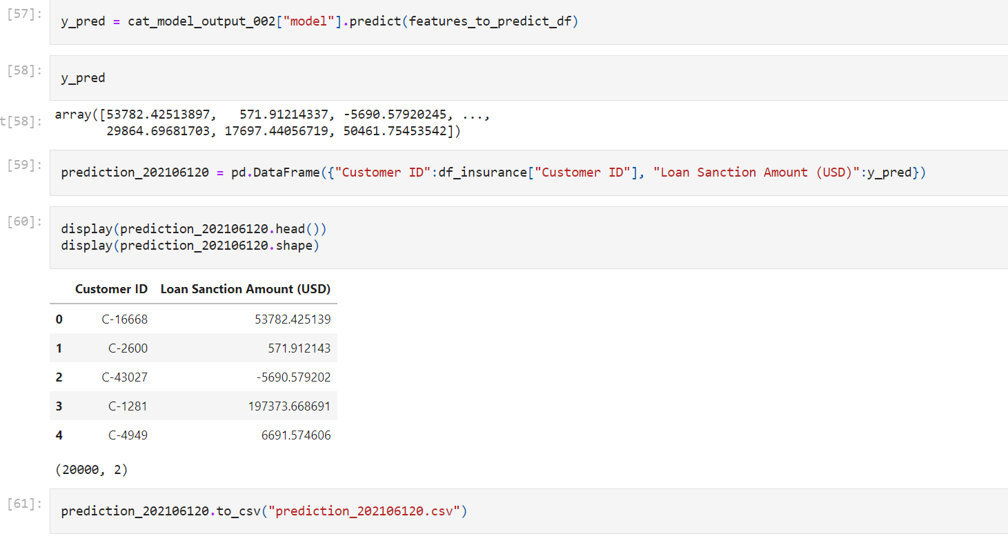
Predict and save results

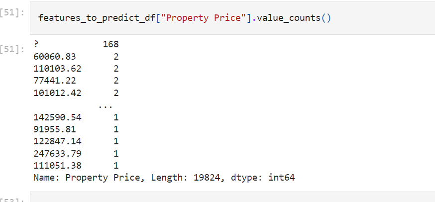
y_pred = cat_model_output_002["model"].predict(features_to_predict_df)
prediction_202106120 = pd.DataFrame({"Customer ID":df_insurance["Customer ID"], "Loan Sanction Amount (USD)":y_pred})
display(prediction_202106120.head())
display(prediction_202106120.shape)
prediction_202106120.to_csv("prediction_202106120.csv")

End Notes

I hope this article has piqued your curiosity and motivated you to try this lesser-known library. Do try out on different datasets and compare the results with an RF model or an XGBoost model.

Good luck! Here is my Linkedin profile in case you want to connect with me. Feel free to ping me on Topmate as well, you can drop me a message with your query. I’ll be happy to be connected. Check out my other articles on data science and analytics here.

Chrisx10 Dmello 10 Jan 2022

Data scientist! Extensively using data mining, data processing algorithms, visualization, statistics and predictive modelling to solve challenging business problems and generate insights.