Beginner’s Guide on Types of Generative Adversarial Networks

Introduction

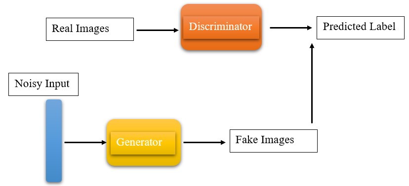
You must have heard of GANs, a cool tech that can create images, music, and more. But what exactly are GANs? Are they part of deep learning? Generative Adversarial Networks, or GANs, are a way to generate data that looks real. They use something called Convolutional Neural Networks (CNNs), which are like super-smart computer brains. In GANs, there are two main players: the Generator and the Discriminator. They’re a bit like two buddies in a game. The Generator makes data, and the Discriminator checks if it’s real or fake. If the Discriminator can’t tell if it’s fake, the Generator is doing a great job. This means the new data is very similar to the original data, although there are exceptions. In this article, we will discuss everything about GANs!

This article was published as a part of the Data Science Blogathon.

The Generator

We know that a neural networks(NN) requires some kind of input to start learning and continue the process. So here the working of the generator is similar to an actual NN. The generator takes in random noise or random vector space. Random noise is nothing but a random array or vector. It converts this noise into a meaningful output so that it looks similar to the original data distributions.

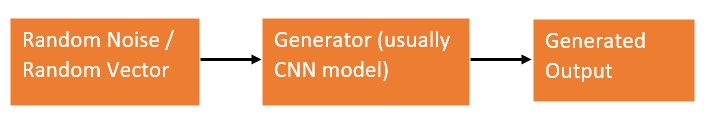
The Generator plays an important role in GAN architecture, with the help of random noise we can get different kinds of output at each run. These outputs will have different combination of multiple features from the original data. But the generator alone can’t do anything. With the help of discriminator, generator carries its work.

The Discriminator

We all trained CNN models on different datasets, Discriminator is similar to them. The discriminator classifies generated images are real or fake. The real images are taken from the original data distribution and the images to be classified are generated by the generator model. The real images are taken from the original data distribution and the images to be classified are generated by the generator model.

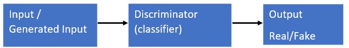
While training the discriminator, it ignores the generator loss and uses only discriminator loss. It updates the weights with the help of backpropagation. We can have different kinds of CNN models which suits our requirements.

Also Read: Why Are Generative Adversarial Networks(GANs) So Famous And How Will GANs Be In The Future?

Simple Generative Adversarial Networks (GAN)

The simple Generative Adversarial Network (GAN) is quite simple, yes it is. While learning about neural networks most of us started with training a classifier on mnist dataset. Similarly, we will do the same here. We will implement image generation using a very simple Generator Discriminator models. I suggest you to use google Colab, which provides free GPU and the training will be faster.

Let’s get started.

Step 1: Import Modules

First, import the required modules

import torch
import torch.nn as nn
import torch.optim as optim
import torchvision
import torchvision.datasets as datasets
from torch.utils.data import DataLoader
import torchvision.transforms as transforms
from torch.utils.tensorboard import SummaryWriter

We will be using PyTorch and from torchvision datasets, we will be using mnist, for preprocessing we will use the transform module from torchvision. Now we will create a class for Discriminator with only linear layers.

class Discriminator(nn.Module):
    def __init__(self, in_features):
        super().__init__()
        self.disc = nn.Sequential(
            nn.Linear(in_features, 128),
            nn.LeakyReLU(0.01),
            nn.Linear(128, 1),
            nn.Sigmoid(),
        )
    def forward(self, x):
        return self.disc(x)

Step 2: Create a Class

Then we will create a class for a generator similar to a discriminator with only linear layers. We will use linear layer, then Leaky ReLu and then linear layer, and finally Tanh. These are simple models compared to different GAN models, but for now, it will do the job.

class Generator(nn.Module):
    def __init__(self, z_dim, img_dim):
        super().__init__()
        self.gen = nn.Sequential(
            nn.Linear(z_dim, 256),
            nn.LeakyReLU(0.01),
            nn.Linear(256, img_dim),
            nn.Tanh(),  # normalize inputs to [-1, 1] so make outputs [-1, 1]
        )
    def forward(self, x):
        return self.gen(x)

Let us initialize the model hyperparameters for training.

device = "cuda" if torch.cuda.is_available() else "cpu"
lr = 3e-4
z_dim = 64
image_dim = 28 * 28 * 1  # 784
batch_size = 32
num_epochs = 50

Step 3: Initialize the Generator and the Discriminator

Then we will initialize the Generator and the Discriminator. To generate random noise for the input to the generator model, we will use torch.randn. This will generate random noise and we will feed it to a generator that generates similar samples to the original datasets.

disc = Discriminator(image_dim).to(device)
gen = Generator(z_dim, image_dim).to(device)
fixed_noise = torch.randn((batch_size, z_dim)).to(device)
transforms = transforms.Compose(
    [transforms.ToTensor(), transforms.Normalize((0.5,), (0.5,)),]) 

Step 4: Download the mnist Dataset

Now we will download the mnist dataset and using torch data loader we will load the mnist dataset, with desired batch size. Then we will declare separate optimizers for generator and discriminator, that is Adam optimizer. We will use BCE loss and then SummaryWriter to save the generated real and fake data and will be saved in the form of tfrecords in logs folder.

dataset = datasets.MNIST(root="dataset/", transform=transforms, download=True)
loader = DataLoader(dataset, batch_size=batch_size, shuffle=True)
opt_disc = optim.Adam(disc.parameters(), lr=lr)
opt_gen = optim.Adam(gen.parameters(), lr=lr)
criterion = nn.BCELoss()
writer_fake = SummaryWriter(f"logs/fake")
writer_real = SummaryWriter(f"logs/real")
step = 0

Step 5: Testing the Model

Now, in a for loop we will declare the training parameters, then generate random noise, and then pass it to the generator, here fake = gen(noise) then initialize loss functions, and then train the generator to give out some samples. Save these samples for visualization.

for epoch in range(num_epochs):
    for batch_idx, (real, _) in enumerate(loader):
        real = real.view(-1, 784).to(device)
        batch_size = real.shape[0]
        ### Train Discriminator: max log(D(x)) + log(1 - D(G(z)))
        noise = torch.randn(batch_size, z_dim).to(device)
        fake = gen(noise)
        disc_real = disc(real).view(-1)
        lossD_real = criterion(disc_real, torch.ones_like(disc_real))
        disc_fake = disc(fake).view(-1)
        lossD_fake = criterion(disc_fake, torch.zeros_like(disc_fake))
        lossD = (lossD_real + lossD_fake) / 2
        disc.zero_grad()
        lossD.backward(retain_graph=True)
        opt_disc.step()
        ### Train Generator: min log(1 - D(G(z)))  max log(D(G(z))
        # where the second option of maximizing doesn't suffer from
        # saturating gradients
        output = disc(fake).view(-1)
        lossG = criterion(output, torch.ones_like(output))
        gen.zero_grad()
        lossG.backward()
        opt_gen.step()
        if batch_idx == 0:
            print(
                f"Epoch [{epoch}/{num_epochs}] Batch {batch_idx}/{len(loader)} 
                       Loss D: {lossD:.4f}, loss G: {lossG:.4f}"
            )
            with torch.no_grad():
                fake = gen(fixed_noise).reshape(-1, 1, 28, 28)
                data = real.reshape(-1, 1, 28, 28)
                img_grid_fake = torchvision.utils.make_grid(fake, normalize=True)
                img_grid_real = torchvision.utils.make_grid(data, normalize=True)
                writer_fake.add_image(
                    "Mnist Fake Images", img_grid_fake, global_step=step
                )
                writer_real.add_image(
                    "Mnist Real Images", img_grid_real, global_step=step
                )
                step += 1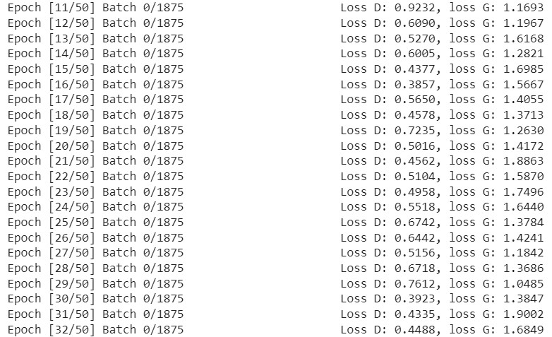

Output

Once the training is completed, it will generate a log folder with tf-records for real and fake images. Using tensoboard we can visualize it to verify the output. Below is the output from the tensorboard.

%load_ext tensorboard

%tensorboard --logdir logs

You can see the model has generated some output that looks quite similar, if you want a better output then train it for more epochs. Once it starts to learn all the features you can see it will generate almost the same images which are present the original dataset. Hope you got some idea of training a GAN model and how the output look like.

Deep Convolutional GAN (DCGAN)

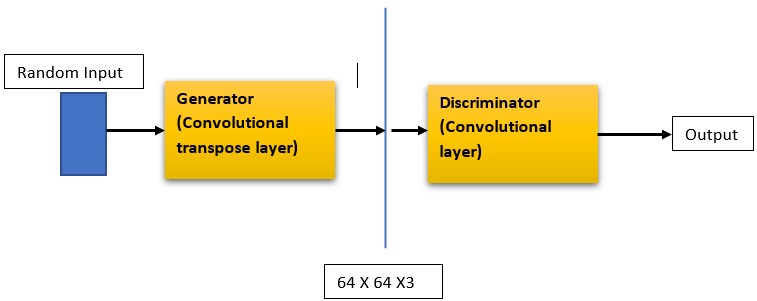
DCGAN is akin to the simple GAN we implemented earlier, but with notable differences. Instead of regular linear layers, DCGAN employs convolutional layers in the discriminator and convolutional-transpose layers in the generator. As outlined in the paper titled ‘UNSUPERVISED REPRESENTATION LEARNING WITH DEEP CONVOLUTIONAL GENERATIVE ADVERSARIAL NETWORKS,’ the generator model incorporates convolutional transpose layers, batch normalization, and ReLU activation. The discriminator block features strided convolution layers, batch normalization, and LeakyReLU activations. Apart from these changes, other aspects remain consistent, except for the loss calculation and model weight initialization. We’ll delve into these specifics as we proceed with the implementation

Let us start the implementation. We will use the same mnist dataset, you can also use other different image datasets like the celeb-face dataset or your custom dataset for image generation.

We will import the required modules. It is pretty much the same as what we used in the previous implementation.

import torch
import torch.nn as nn
import torch.optim as optim
import torchvision
import torchvision.datasets as datasets
import torchvision.transforms as transforms
from torch.utils.data import DataLoader
from torch.utils.tensorboard import SummaryWriter

Then, we will declare a class for the discriminator model which consists of convolutional layers. Here we will define a function _block which takes input channel, output channel, kernel size, stride, and padding. We will use LeakyReLu activation. Our discriminator model consists of very few layers here and it takes the number of image channels and feature size for the input.

class Discriminator(nn.Module):
    def __init__(self, channels_img, features_d):
        super(Discriminator, self).__init__()
        self.disc = nn.Sequential(
            # input: N x channels_img x 64 x 64
            nn.Conv2d(
                channels_img, features_d, kernel_size=4, stride=2, padding=1
            ),
            nn.LeakyReLU(0.2),
            # _block(in_channels, out_channels, kernel_size, stride, padding)
            self._block(features_d, features_d * 2, 4, 2, 1),
            self._block(features_d * 2, features_d * 4, 4, 2, 1),
            self._block(features_d * 4, features_d * 8, 4, 2, 1),
            # After all _block img output is 4x4 (Conv2d below makes into 1x1)
            nn.Conv2d(features_d * 8, 1, kernel_size=4, stride=2, padding=0),
            nn.Sigmoid(),
        )
    def _block(self, in_channels, out_channels, kernel_size, stride, padding):
        return nn.Sequential(
            nn.Conv2d(
                in_channels,
                out_channels,
                kernel_size,
                stride,
                padding,
                bias=False,
            ),
            #nn.BatchNorm2d(out_channels),
            nn.LeakyReLU(0.2),
        )
    def forward(self, x):
        return self.disc(x)

Now, we will create another class for the generator model which consists of transpose convolutional layers. Here we will use the ConvTranspose2d inside _block method with ReLU as activation. This will carry out 2d transposed convolution on the inputs. Here it takes three inputs, the noise dimension, image channel, and the generator feature size.

class Generator(nn.Module):
    def __init__(self, channels_noise, channels_img, features_g):
        super(Generator, self).__init__()
        self.net = nn.Sequential(
            # Input: N x channels_noise x 1 x 1
            self._block(channels_noise, features_g * 16, 4, 1, 0),  # img: 4x4
            self._block(features_g * 16, features_g * 8, 4, 2, 1),  # img: 8x8
            self._block(features_g * 8, features_g * 4, 4, 2, 1),  # img: 16x16
            self._block(features_g * 4, features_g * 2, 4, 2, 1),  # img: 32x32
            nn.ConvTranspose2d(
                features_g * 2, channels_img, kernel_size=4, stride=2, padding=1
            ),
            # Output: N x channels_img x 64 x 64
            nn.Tanh(),
        )
    def _block(self, in_channels, out_channels, kernel_size, stride, padding):
        return nn.Sequential(
            nn.ConvTranspose2d(
                in_channels,
                out_channels,
                kernel_size,
                stride,
                padding,
                bias=False,
            ),
            #nn.BatchNorm2d(out_channels),
            nn.ReLU(),
        )
    def forward(self, x):
        return self.net(x)

Then, we will go for weights initialization. All of the model weights should be initialized randomly which is from a normal distribution with a mean of 0, a std of 0.02. For the below initialize_weights() function, we will pass the model, and then it reinitializes all the convolutional-transpose, convolutional, and batch norm layers. This function should be called immediately after we initialize the generator and the discriminator model. Then we will initialize hyperparameters for our model. that is the learning rate(lr), here we defined a single lr for both generator and discriminator, you can define multiple learning rates for a different model, then initialize the batch size. the number of image channels, here it is 1 because we are using mnist dataset, if you are using other dataset then change it to 3, then initialize noise vector , feature size for generator and discriminator.

def initialize_weights(model):
    for m in model.modules():
        if isinstance(m, (nn.Conv2d, nn.ConvTranspose2d, nn.BatchNorm2d)):
            nn.init.normal_(m.weight.data, 0.0, 0.02)
device = torch.device("cuda" if torch.cuda.is_available() else "cpu")
LEARNING_RATE = 2e-4  # could also use two lrs, one for gen and one for disc
BATCH_SIZE = 128
IMAGE_SIZE = 64
CHANNELS_IMG = 1
NOISE_DIM = 100
NUM_EPOCHS = 50
FEATURES_DISC = 64
FEATURES_GEN = 64

transforms = transforms.Compose(
    [
        transforms.Resize(IMAGE_SIZE),
        transforms.ToTensor(),
        transforms.Normalize(
            [0.5 for _ in range(CHANNELS_IMG)], [0.5 for _ in range(CHANNELS_IMG)]
        ),
    ]
)

After that, we will initialize the mnist dataset, if you’re using different dataset then you should do slight modifications while initializing the dataset, which is shown below in the code. Then we will use DataLoader to load the dataset and then we initialize the Generator and the discriminator model, then we will do weight initialization. We will use Adam optimizer for both models with BCE loss and then using torch SummaryWriter we will have a log folder that contains the details of each epoch.

# If you train on MNIST, remember to set channels_img to 1
dataset = datasets.MNIST(root="dataset/", train=True, transform=transforms,
                       download=True)
# comment mnist above and uncomment below if train on CelebA
#dataset = datasets.ImageFolder(root="celeb_dataset", transform=transforms)
dataloader = DataLoader(dataset, batch_size=BATCH_SIZE, shuffle=True)
gen = Generator(NOISE_DIM, CHANNELS_IMG, FEATURES_GEN).to(device)
disc = Discriminator(CHANNELS_IMG, FEATURES_DISC).to(device)
initialize_weights(gen)
initialize_weights(disc)
opt_gen = optim.Adam(gen.parameters(), lr=LEARNING_RATE, betas=(0.5, 0.999))
opt_disc = optim.Adam(disc.parameters(), lr=LEARNING_RATE, betas=(0.5, 0.999))
criterion = nn.BCELoss()
fixed_noise = torch.randn(32, NOISE_DIM, 1, 1).to(device)
writer_real = SummaryWriter(f"logs/real")
writer_fake = SummaryWriter(f"logs/fake")
step = 0
gen.train()
disc.train()

Then finally the training loop, where we perform basic training steps as we did while implementing Simple GAN.

for epoch in range(NUM_EPOCHS):
    # Target labels not needed! <3 unsupervised
    for batch_idx, (real, _) in enumerate(dataloader):
        real = real.to(device)
        noise = torch.randn(BATCH_SIZE, NOISE_DIM, 1, 1).to(device)
        fake = gen(noise)
        ### Train Discriminator: max log(D(x)) + log(1 - D(G(z)))
        disc_real = disc(real).reshape(-1)
        loss_disc_real = criterion(disc_real, torch.ones_like(disc_real))
        disc_fake = disc(fake.detach()).reshape(-1)
        loss_disc_fake = criterion(disc_fake, torch.zeros_like(disc_fake))
        loss_disc = (loss_disc_real + loss_disc_fake) / 2
        disc.zero_grad()
        loss_disc.backward()
        opt_disc.step()
        ### Train Generator: min log(1 - D(G(z)))  max log(D(G(z))
        output = disc(fake).reshape(-1)
        loss_gen = criterion(output, torch.ones_like(output))
        gen.zero_grad()
        loss_gen.backward()
        opt_gen.step()
        # Print losses occasionally and print to tensorboard
        if batch_idx % 100 == 0:
            print(
                f"Epoch [{epoch}/{NUM_EPOCHS}] Batch {batch_idx}/{len(dataloader)} 
                  Loss D: {loss_disc:.4f}, loss G: {loss_gen:.4f}"
            )
            with torch.no_grad():
                fake = gen(fixed_noise)
                # take out (up to) 32 examples
                img_grid_real = torchvision.utils.make_grid(
                    real[:32], normalize=True
                )
                img_grid_fake = torchvision.utils.make_grid(
                    fake[:32], normalize=True
                )
                writer_real.add_image("Real", img_grid_real, global_step=step)
                writer_fake.add_image("Fake", img_grid_fake, global_step=step)
            step += 1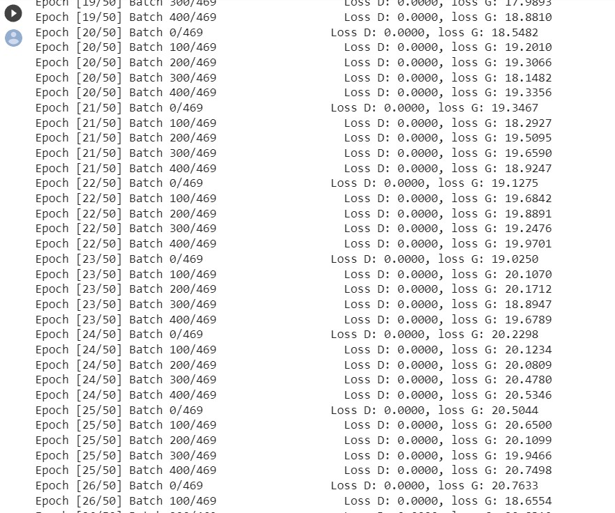

Ones the training is completed you can see the generated output with the help of tensorboard.

%load_ext tensorboard
%tensorboard --logdir logs

The result will look similar to the simple-GAN result, but here the performance will be much better.

That’s it for DCGAN, to get better output train for more epochs and play around with the different hyperparameters. According to the DCGAN paper for stable training follow the below guidelines.

• The pooling layer should be replaced with strided convolution for the discriminator and transpose convolution layer for the generator.
• Using Batchnormalization both in generator and discriminator serves the purpose.
• If you are using fully connected hidden layers then remove them.
• For all the layers in the generator use, ReLU activation and the output layer uses Tanh.
• For all the layers in the discriminator use LeakyReLU activation.

Pix2Pix Conditional GAN

We have seen converting black-n-white images to color images or converting an image from one form to another form, these all can be implemented using GANs. Here we will explore more about Pix2Pix GAN, which is used for the image to image translation. Pix2Pix GAN is a conditional GAN where it learns the feature mapping between the input image to the output image. It was proposed in the Image-to-Image Translation with Conditional Adversarial Networks paper and it has a variety of applications, that is colorizing the image, generating aerial images from the map images, converting sketches to real images, etc. While training the Pix2Pix GAN the dataset must comprise of the input image and its translated output image.

Basic Pix2Pix GAN Model

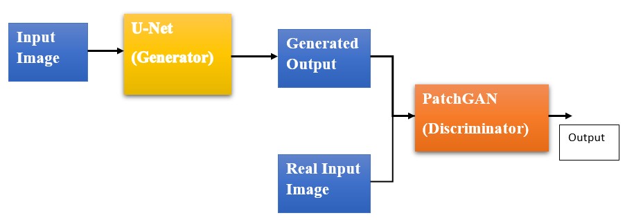
Pix2Pix has a very interesting generator discriminator architecture, the generator uses U-Net architecture and the discriminator uses PatchGAN classifier.

The Generator model does not take random noise, instead, it takes input from input image distribution and the gives out the target image output. The discriminator takes the image and its respective target image and gives probability value for its similarity. Other GANs used the classifier for discriminator, but here we use PatchGAN, which is a deep CNN, classifying the patches in the image as fake or real rather than classifying the entire image.

Let us implement Pix2Pix GAN, don’t worry about the dataset, we will be downloading the dataset directly from Kaggle to our colab workspace. Follow the below steps for downloading the dataset.

!pip install kaggle

Then go to your Kaggle profile and open accounts and scroll down, you will find an option to create API tokens, once you click it, a JSON file will be downloaded, this is required to configure your account on colab so that we can download the dataset.

from google.colab import files
uploaded = files.upload()
for fn in uploaded.keys():
  print('User uploaded file "{name}" with length {length} bytes'.format(
      name=fn, length=len(uploaded[fn])))
# Then move kaggle.json into the folder where the API expects to find it.
!mkdir -p ~/.kaggle/ && mv kaggle.json ~/.kaggle/ && chmod 600 ~/.kaggle/kaggle.json

Once you run the above code upload the API JSON file and then copy the API command for the dataset, paste it is the cell, and run it. This will download the dataset and the unzip it.

!kaggle datasets download -d ktaebum/anime-sketch-colorization-pair
!unzip /content/anime-sketch-colorization-pair.zip

First, we will declare some of the hyperparameters and preprocessing steps required for the model and the dataset. We will use the albumentations library to perform the preprocessing steps. the hyperparameters include learning rate, batch size, number of workers, image size, image channel, number of epochs, etc.

!pip install -U git+https://github.com/albu/albumentations --no-cache-dir

Execute and Restart the Colab Runtime

import torch
import albumentations as A
from albumentations.pytorch import ToTensorV2

DEVICE = "cuda" if torch.cuda.is_available() else "cpu"
TRAIN_DIR = "/content/data/train"
VAL_DIR = "/content/data/val"
LEARNING_RATE = 2e-4
BATCH_SIZE = 16
NUM_WORKERS = 2
IMAGE_SIZE = 256
CHANNELS_IMG = 3
L1_LAMBDA = 100
LAMBDA_GP = 10
NUM_EPOCHS = 500
LOAD_MODEL = False
SAVE_MODEL = False
CHECKPOINT_DISC = "disc.pth.tar"
CHECKPOINT_GEN = "gen.pth.tar"
both_transform = A.Compose(
 [A.Resize(width=256, height=256),], additional_targets={"image0": "image"},
)

transform_only_input = A.Compose(
 [
 A.HorizontalFlip(p=0.5),
A.ColorJitter(p=0.2),
A.Normalize(mean=[0.5, 0.5, 0.5], std=[0.5, 0.5, 0.5], max_pixel_value=255.0,),
ToTensorV2(),
]
)

transform_only_mask = A.Compose(
 [
 A.Normalize(mean=[0.5, 0.5, 0.5], std=[0.5, 0.5, 0.5], max_pixel_value=255.0,),
ToTensorV2(),
]
)

Write a Small Class to Apply the Preprocessing Steps

Now we have the dataset we will write a small class to apply the preprocessing steps to the dataset, here we will make the dataset compatible with our model. Below is the class AnimeDataset() which takes dataset path as input and then it performs augmentations of the input and target images and returns it.

class AnimeDataset(Dataset):
    def __init__(self, root_dir):
        self.root_dir = root_dir
        self.list_files = os.listdir(self.root_dir)
    def __len__(self):
        return len(self.list_files)
    def __getitem__(self, index):
        img_file = self.list_files[index]
        img_path = os.path.join(self.root_dir, img_file)
        image = np.array(Image.open(img_path))
        input_image = image[:, :600, :]
        target_image = image[:, 600:, :]
        augmentations = both_transform(image=input_image, image0=target_image)
        input_image = augmentations["image"]
        target_image = augmentations["image0"]
        input_image = transform_only_input(image=input_image)["image"]
        target_image = transform_only_mask(image=target_image)["image"]
        return input_image, target_image

Have a Test Run on the Dataset

To verify if the above steps are working fine, we will have a test run on the dataset. Execute the below cell and you will see the shape of the image and the source and target image are being saved as test_run_x.png and test_run_y.png respectively on the workspace. You can stop this running cell, once you see these outputs.

dataset = AnimeDataset("/content/data/train/")
loader = DataLoader(dataset, batch_size=5)
for x, y in loader:
    print(x.shape)
    save_image(x, "test_run_x.png")
    save_image(y, "test_run_y.png")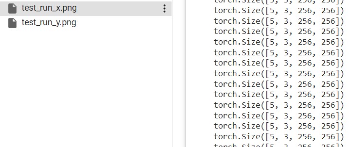

Define the Discriminator Model

Now, let us define the discriminator model. As we know it is a PatchGAN classifies if each patch in the image is real or fake, below are the features of the discriminator.

• The discriminator is made up of blocks, which have: Convolution layer -> Batch normalization -> Leaky ReLU activation.
• After the last layer, the shape of the output is (batch_size, 30, 30, 1).
• Each 70 x 70 region of the input image is classified by each 30 x 30 image patch output.

import torch
import torch.nn as nn

class CNNBlock(nn.Module):
def __init__(self, in_channels, out_channels, stride):
super(CNNBlock, self).__init__()
 self.conv = nn.Sequential(
 nn.Conv2d(
 in_channels, out_channels, 4, stride, 1, bias=False, padding_mode="reflect"
),
nn.BatchNorm2d(out_channels),
nn.LeakyReLU(0.2),
)

 def forward(self, x):
return self.conv(x)


class Discriminator(nn.Module):
def __init__(self, in_channels=3, features=[64, 128, 256, 512]):
super().__init__()
 self.initial = nn.Sequential(
 nn.Conv2d(
 in_channels * 2,
features[0],
kernel_size=4,
stride=2,
padding=1,
padding_mode="reflect",
),
nn.LeakyReLU(0.2),
)

 layers = []
 in_channels = features[0]
 for feature in features[1:]:
layers.append(
 CNNBlock(in_channels, feature, stride=1 if feature == features[-1] else 2),
)
 in_channels = feature

layers.append(
 nn.Conv2d(
 in_channels, 1, kernel_size=4, stride=1, padding=1, padding_mode="reflect"
),
)

 self.model = nn.Sequential(*layers)

 def forward(self, x, y):
x = torch.cat([x, y], dim=1)
 x = self.initial(x)
 x = self.model(x)
 return x

Generating Another Class

Now let us define the generator class, which is a u-net architecture. Here we will define a class called Block() use it inside the generator class. Below you can get a better picture of the number of layers, activation functions, and features used in the generator.

import torch
import torch.nn as nn

class Block(nn.Module):
def __init__(self, in_channels, out_channels, down=True, act="relu", use_dropout=False):
super(Block, self).__init__()
 self.conv = nn.Sequential(
 nn.Conv2d(in_channels, out_channels, 4, 2, 1, bias=False, padding_mode="reflect")
 if down
else nn.ConvTranspose2d(in_channels, out_channels, 4, 2, 1, bias=False),
nn.BatchNorm2d(out_channels),
nn.ReLU() if act == "relu" else nn.LeakyReLU(0.2),
)

 self.use_dropout = use_dropout
self.dropout = nn.Dropout(0.5)
 self.down = down

def forward(self, x):
x = self.conv(x)
 return self.dropout(x) if self.use_dropout else x

class Generator(nn.Module):
def __init__(self, in_channels=3, features=64):
super().__init__()
 self.initial_down = nn.Sequential(
 nn.Conv2d(in_channels, features, 4, 2, 1, padding_mode="reflect"),
nn.LeakyReLU(0.2),
)
 self.down1 = Block(features, features * 2, down=True, act="leaky", use_dropout=False)
 self.down2 = Block(
 features * 2, features * 4, down=True, act="leaky", use_dropout=False
)
 self.down3 = Block(
 features * 4, features * 8, down=True, act="leaky", use_dropout=False
)
 self.down4 = Block(
 features * 8, features * 8, down=True, act="leaky", use_dropout=False
)
 self.down5 = Block(
 features * 8, features * 8, down=True, act="leaky", use_dropout=False
)
 self.down6 = Block(
 features * 8, features * 8, down=True, act="leaky", use_dropout=False
)
 self.bottleneck = nn.Sequential(
 nn.Conv2d(features * 8, features * 8, 4, 2, 1), nn.ReLU()
 )

 self.up1 = Block(features * 8, features * 8, down=False, act="relu", use_dropout=True)
 self.up2 = Block(
 features * 8 * 2, features * 8, down=False, act="relu", use_dropout=True
)
 self.up3 = Block(
 features * 8 * 2, features * 8, down=False, act="relu", use_dropout=True
)
 self.up4 = Block(
 features * 8 * 2, features * 8, down=False, act="relu", use_dropout=False
)
 self.up5 = Block(
 features * 8 * 2, features * 4, down=False, act="relu", use_dropout=False
)
 self.up6 = Block(
 features * 4 * 2, features * 2, down=False, act="relu", use_dropout=False
)
 self.up7 = Block(features * 2 * 2, features, down=False, act="relu", use_dropout=False)
 self.final_up = nn.Sequential(
 nn.ConvTranspose2d(features * 2, in_channels, kernel_size=4, stride=2, padding=1),
nn.Tanh(),
)

 def forward(self, x):
d1 = self.initial_down(x)
 d2 = self.down1(d1)
 d3 = self.down2(d2)
 d4 = self.down3(d3)
 d5 = self.down4(d4)
 d6 = self.down5(d5)
 d7 = self.down6(d6)
 bottleneck = self.bottleneck(d7)
 up1 = self.up1(bottleneck)
 up2 = self.up2(torch.cat([up1, d7], 1))
 up3 = self.up3(torch.cat([up2, d6], 1))
 up4 = self.up4(torch.cat([up3, d5], 1))
 up5 = self.up5(torch.cat([up4, d4], 1))
 up6 = self.up6(torch.cat([up5, d3], 1))
 up7 = self.up7(torch.cat([up6, d2], 1))
 return self.final_up(torch.cat([up7, d1], 1))

Now we will define some of the utility functions like saving the checkpoint, loading the checkpoint, and saving some of the generated output. We will define a function named save_some_example() here it will take the generator model, validation loader, epoch number, and the folder path as the inputs arguments, then we will use save_img from torchvision to save the generated output.

Define Another Function

Then, we will define another function to save the checkpoints, this function will take the model, its optimizer, and the file name for input arguments and we will save the model dict using torch.save(). Similarly for loading the checkpoints we can use torch.load() and then load the model state dict. These are the utility functions.

from torchvision.utils import save_image

def save_some_examples(gen, val_loader, epoch, folder):
x, y = next(iter(val_loader))
 x, y = x.to(DEVICE), y.to(DEVICE)
 gen.eval()
 with torch.no_grad():
y_fake = gen(x)
 y_fake = y_fake * 0.5 + 0.5 # remove normalization#
save_image(y_fake, folder + f"/y_gen_{epoch}.png")
 save_image(x * 0.5 + 0.5, folder + f"/input_{epoch}.png")
 if epoch == 1:
save_image(y * 0.5 + 0.5, folder + f"/label_{epoch}.png")
 gen.train()

def save_checkpoint(model, optimizer, filename="my_checkpoint.pth.tar"):
print("=> Saving checkpoint")
 checkpoint = {
 "state_dict": model.state_dict(),
"optimizer": optimizer.state_dict(),
}
 torch.save(checkpoint, filename)


def load_checkpoint(checkpoint_file, model, optimizer, lr):
print("=> Loading checkpoint")
 checkpoint = torch.load(checkpoint_file, map_location=DEVICE)
 model.load_state_dict(checkpoint["state_dict"])
 optimizer.load_state_dict(checkpoint["optimizer"])

 # If we don't do this then it will just have learning rate of old checkpoint
# and it will lead to many hours of debugging :
for param_group in optimizer.param_groups:
param_group["lr"] = lr

We are all set to train our Pix2Pix GAN model now. First we will import the required libraries.

import torch
import torch.nn as nn
import torch.optim as optim
from torch.utils.data import DataLoader
from tqdm import tqdm
from torchvision.utils import save_image
torch.backends.cudnn.benchmark = True

Now, we will define the train function, this function will take discriminator, generator, data loader, generator optimizer, discriminator optimizer, loss functions, and generator scaler and discriminator scaler. First, we will loop through the data loader and then send all the parameters to GPU, then we will send the desired data to the generator and the discriminator and obtain loss values for both.

def train_fn(
    disc, gen, loader, opt_disc, opt_gen, l1_loss, bce, g_scaler, d_scaler,
):
    loop = tqdm(loader, leave=True)
    for idx, (x, y) in enumerate(loop):
        x = x.to(DEVICE)
        y = y.to(DEVICE)
        # Train Discriminator
        with torch.cuda.amp.autocast():
            y_fake = gen(x)
            D_real = disc(x, y)
            D_real_loss = bce(D_real, torch.ones_like(D_real))
            D_fake = disc(x, y_fake.detach())
            D_fake_loss = bce(D_fake, torch.zeros_like(D_fake))
            D_loss = (D_real_loss + D_fake_loss) / 2
        disc.zero_grad()
        d_scaler.scale(D_loss).backward()
        d_scaler.step(opt_disc)
        d_scaler.update()
        # Train generator
        with torch.cuda.amp.autocast():
            D_fake = disc(x, y_fake)
            G_fake_loss = bce(D_fake, torch.ones_like(D_fake))
            L1 = l1_loss(y_fake, y) * L1_LAMBDA
            G_loss = G_fake_loss + L1

opt_gen.zero_grad()
 g_scaler.scale(G_loss).backward()
 g_scaler.step(opt_gen)
 g_scaler.update()

 if idx % 10 == 0:
loop.set_postfix(
 D_real=torch.sigmoid(D_real).mean().item(),
D_fake=torch.sigmoid(D_fake).mean().item(),
)

Then the main function, here we will initialize the generator and discriminator, the optimizers for them as well as the loss functions. If you want to resume the training set LOAD_MODEL variable to True, we will initialize our train data and create a DataLoader for it, similar for validation data as well and at the end the model will be saved and the generated examples will also be saved in a folder. Run the main() function.

def main():
    disc = Discriminator(in_channels=3).to(DEVICE)
    gen = Generator(in_channels=3, features=64).to(DEVICE)
    opt_disc = optim.Adam(disc.parameters(), lr=LEARNING_RATE, betas=(0.5, 0.999),)
    opt_gen = optim.Adam(gen.parameters(), lr=LEARNING_RATE, betas=(0.5, 0.999))
    BCE = nn.BCEWithLogitsLoss()
    L1_LOSS = nn.L1Loss()
    if LOAD_MODEL:
        load_checkpoint(
            CHECKPOINT_GEN, gen, opt_gen, LEARNING_RATE,
        )
        load_checkpoint(
            CHECKPOINT_DISC, disc, opt_disc, LEARNING_RATE,
        )
    train_dataset = AnimeDataset(root_dir=TRAIN_DIR)
    train_loader = DataLoader(
        train_dataset,
        batch_size=BATCH_SIZE,
        shuffle=True,
        num_workers=NUM_WORKERS,
    )
    g_scaler = torch.cuda.amp.GradScaler()
    d_scaler = torch.cuda.amp.GradScaler()
    val_dataset = AnimeDataset(root_dir=VAL_DIR)
    val_loader = DataLoader(val_dataset, batch_size=1, shuffle=False)
    for epoch in range(NUM_EPOCHS):
        train_fn(
            disc, gen, train_loader, opt_disc, opt_gen, L1_LOSS, BCE, g_scaler, d_scaler,
        )
        if SAVE_MODEL and epoch % 5 == 0:
            save_checkpoint(gen, opt_gen, filename=CHECKPOINT_GEN)
            save_checkpoint(disc, opt_disc, filename=CHECKPOINT_DISC)
        save_some_examples(gen, val_loader, epoch, folder="/content/drive/MyDrive/pix2pix_output")
main()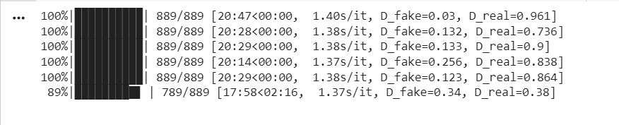

While the training is in progress, we can see the intermediate outputs, below is a snapshot of it when the model was in 478th epoch.

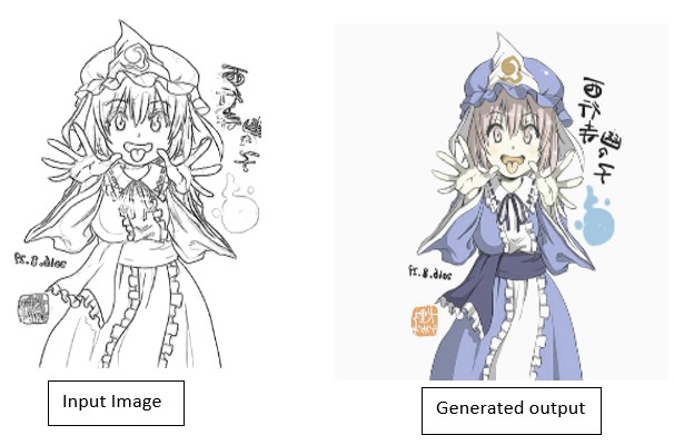
The output is pretty much good, but if you train it for some more time, eventually it gets better.  Then you can pass your own sketches while inferencing to get colorized images.  That’s it for Pix2Pix GAN.

Cycle Generative Adversarial Networks

Cycle GAN is very much similar to Pix2Pix GAN except for the training method and its architecture. It is also mainly used for image to image translation. The Cycle GAN architecture seems to be complex, since it takes care lot of image mapping and feature generation.

In Cycle GAN we use a cycle consistency loss which helps us to train the model without the need for paired data as we did in Pix2Pix. It can easily translate the image from one domain to another without the requirement of one-to-one mapping. Cycle consistency loss checks if the result is close to the original input, here if we consider an image of a horse translated to zebra, and then again translate that zebra image to horse image, the loss between this translated image and the original image must be less. This is what cycle consistency loss does.

Here, it uses two generator and two discriminator. if we consider two sources A and B, one generator generates image for source A and the other one generates image for source B.

• Generator-A >> Source-A
• Generator-B >> Source-B

The generator models take inputs from each other. Generator-A takes input image from Source-B and Generator-B takes input image from Source-A.

• Source -B >> Generator-A >> Source -A
• Source -A >> Generator-B >> Source -B

Each generator model has a discriminator model. The first discriminator model takes generated images from Generator-A and real images from Source-A and then, it runs classification for real or fake. The second discriminator model takes generated images from Generator-B and real images from Source -B and runs classification for real or fake.

• Source -A >> Discriminator-A >> [Real/Fake]
• Source -B >> Generator-A >> Discriminator-A >> [Real/Fake]
• Source -B >> Discriminator-B >> [Real/Fake]
• Source -A >> Generator-B >> Discriminator-B >> [Real/Fake]

This is the basic how Cycle GAN works. For implementation you can refer this

Applications of Generative Adversarial Networks

GANs have variety of applications in different fields.

• Generate fun Cartoon Characters
• Generate samples for the Image Datasets
• Generate Human Faces
• Image-to-Image Translation
• Generate high quality Realistic Photographs
• Text-to-Image Translation
• Face Frontal View Generation
• Generate Human Poses
• Convert Photos to Emojis
• Face Aging
• Blending the Images
• Super Resolution
• Clothing Translation
• Video Prediction
• 3D Object Generation
• Image colorization

And many more.

Conclusion

These are the basic types of Generative Adversarial Networks. It is still evolving and there are many different varieties with more complex models of GAN which you can explore. You can build your image generation model or if you have fewer image data you can generate more using GAN, which pretty good results.

You can try the above implementations with different image datasets and implement some cool applications.

All the notebooks are available here.

References:

• Unsupervised Representation Learning with Deep Convolutional Generative Adversarial Networks
• Image-to-Image Translation with Conditional Adversarial Networks
• Unpaired Image-to-Image Translation using Cycle-Consistent Adversarial Networks

Thank You!

Frequently Asked Questions

The media shown in this article is not owned by Analytics Vidhya and are used at the Author’s discretion.

Syed Abdul Gaffar Shakhadri 31 Oct 2023

I am an enthusiastic AI developer, I love playing with different problems and building solutions.