Stock price using LSTM and its implementation

This article was published as a part of the Data Science Blogathon

Introduction

Dataset

https://github.com/PacktPublishing/Learning-Pandas-Second-Edition/blob/master/data/goog.csv

Implementation of LSTM on stocks data

Reading data:

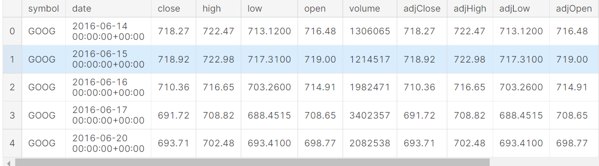
gstock_data = pd.read_csv('data.csv')
gstock_data .head()

Exploring Dataset:

The dataset contains 14 columns associated with time series like the date and the different variables like close, high, low and volume. We will use opening and closing values for our experimentation of time series with LSTM.

gstock_data = gstock_data [['date','open','close']] 
gstock_data ['date'] = pd.<a onclick="parent.postMessage({'referent':'.pandas.to_datetime'}, '*')">to_datetime(gstock_data ['date'].apply(lambda x: x.split()[0])) 
gstock_data .set_index('date',drop=True,inplace=True) 
gstock_data .head()

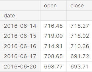
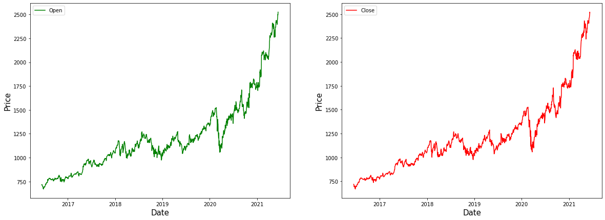
We have performed a few feature extraction here. We take the dates alone from the overall date variable. Now we can be using matplotlib to visualize the available data and see how our price values in data are being displayed. The green colour was used to visualize the open variable for the price-date graph, and for the closing variable, we used red colour.

fg, ax =plt.<a onclick="parent.postMessage({'referent':'.matplotlib.pyplot.subplots'}, '*')">subplots(1,2,figsize=(20,7))
ax[0].plot(gstock_data ['open'],label='Open',color='green')
ax[0].set_xlabel('Date',size=15)
ax[0].set_ylabel('Price',size=15)
ax[0].legend()
ax[1].plot(gstock_data ['close'],label='Close',color='red')
ax[1].set_xlabel('Date',size=15)
ax[1].set_ylabel('Price',size=15)
ax[1].legend()
fg.show()

Data Pre-processing:

We must pre-process this data before applying stock price using LSTM. Transform the values in our data with help of the fit_transform function. Min-max scaler is used for scaling the data so that we can bring all the price values to a common scale. We then use 80 % data for training and the rest 20% for testing and assign them to separate variables.

from sklearn.preprocessing import MinMaxScaler
Ms = MinMaxScaler()
gstock_data [gstock_data .columns] = Ms.fit_transform(gstock_data )

training_size = round(len(gstock_data ) * 0.80)

train_data = gstock_data [:training_size]
test_data  = gstock_data [training_size:]

Splitting data for training:

A function is created so that we can create the sequence for training and testing.

def create_sequence(<a onclick="parent.postMessage({'referent':'.kaggle.usercode.22406117.81090952.create_sequence..dataset'}, '*')">dataset):
  <a onclick="parent.postMessage({'referent':'.kaggle.usercode.22406117.81090952.create_sequence..sequences'}, '*')">sequences = []
  <a onclick="parent.postMessage({'referent':'.kaggle.usercode.22406117.81090952.create_sequence..labels'}, '*')">labels = []

  <a onclick="parent.postMessage({'referent':'.kaggle.usercode.22406117.81090952.create_sequence..start_idx'}, '*')">start_idx = 0

  for <a onclick="parent.postMessage({'referent':'.kaggle.usercode.22406117.81090952.create_sequence..stop_idx'}, '*')">stop_idx in range(50,len(<a onclick="parent.postMessage({'referent':'.kaggle.usercode.22406117.81090952.create_sequence..dataset'}, '*')">dataset)): 
    <a onclick="parent.postMessage({'referent':'.kaggle.usercode.22406117.81090952.create_sequence..sequences'}, '*')">sequences.append(<a onclick="parent.postMessage({'referent':'.kaggle.usercode.22406117.81090952.create_sequence..dataset'}, '*')">dataset.iloc[<a onclick="parent.postMessage({'referent':'.kaggle.usercode.22406117.81090952.create_sequence..start_idx'}, '*')">start_idx:<a onclick="parent.postMessage({'referent':'.kaggle.usercode.22406117.81090952.create_sequence..stop_idx'}, '*')">stop_idx])
    <a onclick="parent.postMessage({'referent':'.kaggle.usercode.22406117.81090952.create_sequence..labels'}, '*')">labels.append(<a onclick="parent.postMessage({'referent':'.kaggle.usercode.22406117.81090952.create_sequence..dataset'}, '*')">dataset.iloc[<a onclick="parent.postMessage({'referent':'.kaggle.usercode.22406117.81090952.create_sequence..stop_idx'}, '*')">stop_idx])
    <a onclick="parent.postMessage({'referent':'.kaggle.usercode.22406117.81090952.create_sequence..start_idx'}, '*')">start_idx += 1
  return (np.<a onclick="parent.postMessage({'referent':'.numpy.array'}, '*')">array(<a onclick="parent.postMessage({'referent':'.kaggle.usercode.22406117.81090952.create_sequence..sequences'}, '*')">sequences),np.<a onclick="parent.postMessage({'referent':'.numpy.array'}, '*')">array(<a onclick="parent.postMessage({'referent':'.kaggle.usercode.22406117.81090952.create_sequence..labels'}, '*')">labels))

train_seq, train_label = create_sequence(train_data)
test_seq, test_label = create_sequence(test_data)

Implementation of our LSTM model:

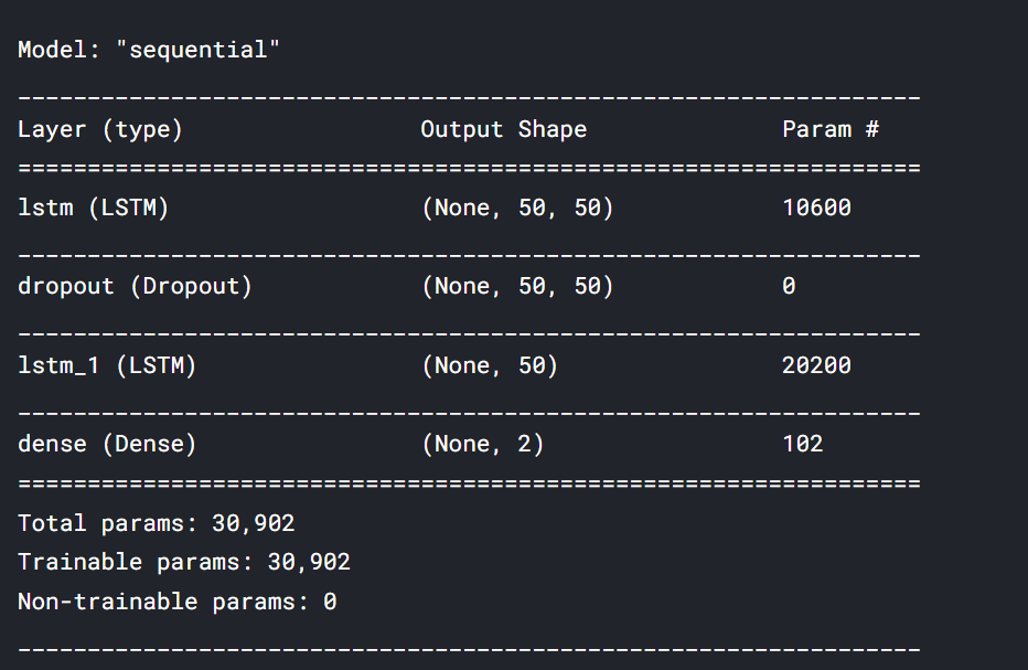
In the next step, we create our LSTM model.  In this article, we will use the Sequential model imported from Keras and required libraries are imported.

from keras.models import Sequential
from keras.layers import Dense, Dropout, LSTM, Bidirectional

We use two LSTM layers in our model and implement drop out in between for regularization. The number of units assigned in the LSTM parameter is fifty. with a dropout of 10 %. Mean squared error is the loss function for optimizing the problem with adam optimizer. Mean absolute error is the metric used in our LSTM network as it is associated with time-series data

model = Sequential()
model.add(LSTM(units=50, return_sequences=True, input_shape = (train_seq.shape[1], train_seq.shape[2])))

model.add(Dropout(0.1)) 
model.add(LSTM(units=50))

model.add(Dense(2))

model.compile(loss='mean_squared_error', optimizer='adam', metrics=['mean_absolute_error'])

model.summary()

model.fit(train_seq, train_label, epochs=80,validation_data=(test_seq, test_label), verbose=1)

test_predicted = model.predict(test_seq)

test_inverse_predicted = MMS.inverse_transform(test_predicted)

Visualization:

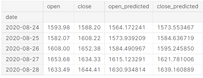
After fitting the data with our model we use it for prediction. We must use inverse transformation to get back the original value with the transformed function. Now we can use this data to visualize the prediction.

# Merging actual and predicted data for better visualization
gs_slic_data = pd.concat([gstock_data .iloc[-202:].copy(),pd.DataFrame(test_inverse_predicted,columns=['open_predicted','close_predicted'],index=gstock_data .iloc[-202:].index)], axis=1)

gs_slic_data[['open','close']] = MMS.inverse_transform(gs_slic_data[['open','close']])

gs_slic_data.head()

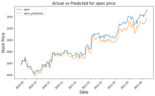
gs_slic_data[['open','open_predicted']].plot(figsize=(10,6))
plt.<a onclick="parent.postMessage({'referent':'.matplotlib.pyplot.xticks'}, '*')">xticks(rotation=45)
plt.<a onclick="parent.postMessage({'referent':'.matplotlib.pyplot.xlabel'}, '*')">xlabel('Date',size=15)
plt.<a onclick="parent.postMessage({'referent':'.matplotlib.pyplot.ylabel'}, '*')">ylabel('Stock Price',size=15)
plt.<a onclick="parent.postMessage({'referent':'.matplotlib.pyplot.title'}, '*')">title('Actual vs Predicted for open price',size=15)
plt.<a onclick="parent.postMessage({'referent':'.matplotlib.pyplot.show'}, '*')">show()

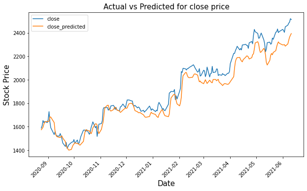
gs_slic_data[['close','close_predicted']].plot(figsize=(10,6))
plt.<a onclick="parent.postMessage({'referent':'.matplotlib.pyplot.xticks'}, '*')">xticks(rotation=45)
plt.<a onclick="parent.postMessage({'referent':'.matplotlib.pyplot.xlabel'}, '*')">xlabel('Date',size=15)
plt.<a onclick="parent.postMessage({'referent':'.matplotlib.pyplot.ylabel'}, '*')">ylabel('Stock Price',size=15)
plt.<a onclick="parent.postMessage({'referent':'.matplotlib.pyplot.title'}, '*')">title('Actual vs Predicted for close price',size=15)
plt.<a onclick="parent.postMessage({'referent':'.matplotlib.pyplot.show'}, '*')">show()

Conclusion

In this article, we explored LSTM and stock price using LSTM. We then visualized the opening and closing price value after using LSTM.

Reference:

1. https://the-learning-machine.com/article/dl/long-short-term-memory
2. https://www.kaggle.com/amarsharma768/stock-price-prediction-using-lstm/notebook

About Me: I am a Research Student interested in the field of Deep Learning and Natural Language Processing and pursuing post-graduation in Artificial Intelligence.

Image Source:

1. Preview Image: https://www.analyticssteps.com/blogs/introduction-time-series-analysis-time-series-forecasting-machine-learning-methods-models

Feel free to connect with me on:

1. Linkedin: https://www.linkedin.com/in/siddharth-m-426a9614a/
2. Github: https://github.com/Siddharth1698

The media shown in this article is not owned by Analytics Vidhya and are used at the Author’s discretion. 

Siddharth M 06 Dec 2021