What’s Happening in Backpropagation? A Behind the Scenes Look at Deep Learning
Training the Black Box
The previous article was all about forward propagation in neural networks, how it works and why it works. One of the important entities in forward propagation is weights. We saw how tuning the weights can take advantage of the non-linearity introduced in each layer to leverage the resultant output. As we said we are going to randomly initialize the weights and biases and let the network learn these weights over time. Now comes the most important question. how are these weights going to be updated? how are the right weights and biases, that optimize the performance of the network to approximate the original relationship between x and y, going to be learned?
A peek into Gradient Descent
Before we go further, I hope you are familiar with Gradient Descent. If not, Let’s have a quick peek. Gradient Descent is an algorithm that is used for the minimization of a function with no local minima.
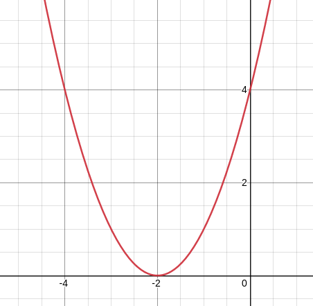
Let us consider an example function as shown in fig 1.1. This is nothing but y = (x + 2)². We know, just by looking at this function that the value of y will be minimum when x = -2. But, is there any way where we can make an algorithm learn this through an iterative fashion?
Let’s randomly initialize the value for x and then iteratively change the value of x in a way, so that value of y reaches a minimum. Let’s say that the value of x is 0. Then, y will be 4. find the slope or tangent of y with respect to x (dy/dx) at x = 0. The answer is 4 (a positive number). Do the same process for x = -4. you’ll notice that the slope or tangent of y with respect to x (dy/dx) at x = -4 is -4 (a negative number).
we know that the value of x needs to be reduced when it is greater than -2 and it needs to be increased when it is lesser than -2.
Using basic differential calculus, we come to the conclusion that whenever the value of x needs to be reduced, dy/dx is a positive number. whenever it needs to be increased, dy/dx is a negative number. If you don’t believe me, you can go ahead and try testing this theory on any function with any value for x, and it also makes sense logically, if you think about it for some time.
Hence, we can use differentiation to find the direction we need to move the value of x in order to reduce y. That direction is nothing but the direction opposite to the slope or tangent at that point. One more thing to acknowledge is that we’ll only be moving x in that direction in tiny magnitude so as to ensure that it doesn’t overshoot and gets away from the global minima, to the other side. On repeating this process, again and again, we’ll finally be able to reach x = -2 and y = 0, which is what we want.
Understanding gradient descent is the cornerstone to understanding backpropagation. If you do not understand gradient descent properly, please take your own time in doing so. Here’s a video that’ll help you if you haven’t understood the idea behind gradient descent already.
Backpropagation: Basic Idea Behind It
If you are familiar with forward propagation, you already know that we randomly initialize the weights and biases in the network and use that to make predictions, just like how we randomly initialized x in the previous section. we take these predictions made by our neural network and use some sort of metric to measure the deviation between the actual target and our model’s output ( This is nothing but the loss function ).
We then proceed to differentiate the loss function with respect to each and every individual weight in the network, similar to how we differentiated y with respect to x in the previous example. Once this is done, we update the weights in the direction opposite to the differentiated term.
Derivations and Proofs
What I cannot create, I do not understand – Richard P. Feynman
I thought backpropagation was one of those things in my life that I would never be able to comprehend, until I created a neural network and trained it on my own, from scratch ( without using deep learning libraries ).
I realized I was fussing over nothing once the algorithm worked and the network was able to accurately approximate the relationship between x and y.
Let’s consider an example neural network and derive the entire formula for backpropagation.
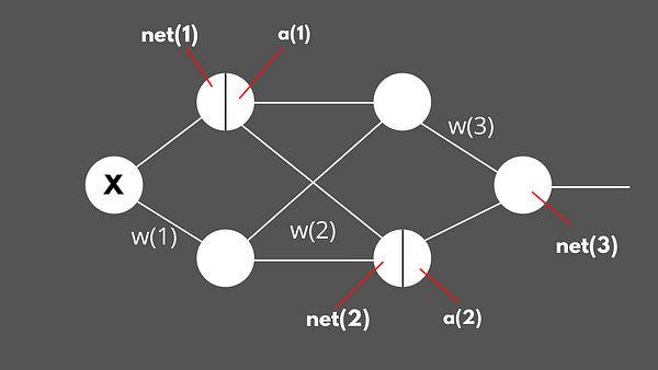
before going head-on into backpropagation, it would be a good idea to define the notations for forward propagation and see how neural this neural network makes it’s predictions.
Forward Propagation
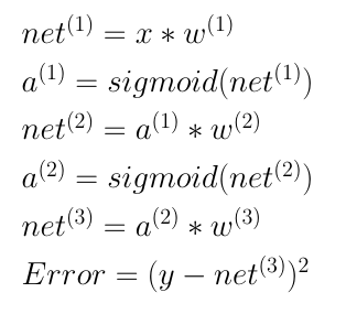
Everything right from the input X to output Net(3) is a matrix in fig 2.2.
I didn’t consider the bias terms just for the sake of simplicity. Once the updation of the weights are interpreted well, it is not very difficult to do the same for the biases. Except that, The above 6 lines are pretty much self explanatory if you are well versed with forward propagation.
Backpropagation
Objective: To find the derivatives for the loss or error with respect to every single weight in the network, and update these weights in the direction opposite to their respected derivatives so as to move towards the global or local minima of the cost or error function.
Before we begin, One special feature of the sigmoid activation function is that its derivative is very easy to calculate.
derivative of sigmoid(x) = sigmoid(x) * (1 — sigmoid(x)).
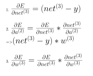
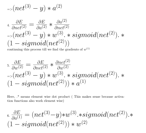
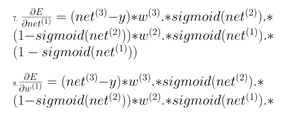
In order to find how the error changes with weights of the first layer, one needs to know how the error changes with the ouptut from the first layer and that requires how the error changes with the activation from the first layer and so on ( Chain Rule ). Hence, we need to start from the final layer and backpropagate the derivatives from there and thus the name, Backpropagation.
In some online courses or slides, you might see the symbol delta that is commonly used for representing errors in each layer. That’s just done for better notation purposes. But, the process is the same.
Update Weights
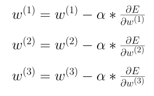
We finally update the weights using the above formula. Alpha is a small number that is used to reduce the magnitude of the updation so that the new weights help the loss slowly reach the global minimum instead of exploding it to the other side and thus, increasing the loss.
Proof this works
I created a custom dataset using a neural network with random weights and used an entirely different neural network with a different number of layers and neurons per layer to learn weights in such a way that the relationship between the dependent and independent variable is accurately mimicked.
Some final Analysis and Conclusion
If you are a beginner to backpropagation, you can think of it as the implementation of gradient descent with chain rule, as there are multiple layers present. The single most important thing is to find out the direction in which the weights need to be moved so as to reach the global minima of the cost function. Differential calculus helps us find this direction (reduce weight if the derivative is +ve and increase if the derivative is -ve).
Since we are only concerned so much about the direction, is it okay to remove the sigmoid terms from the equation, as sigmoid(x) (1- sigmoid(x)) will always lie between 0 and 0.5 for any value of x ? turns out this is the method adopted in Build your own neural network. This is done so as an alternative to an increasing the learning rate.
Backpropagation is a standard process that drives the learning process in any type of neural network. Based on how the forward propagation differs for different neural networks, each type of network is also used for a variety of different use cases. But at the end of the day, when it comes to actually updating the weights, we are going to use the same concept of partial derivatives and chain rule to accomplish that, and reduce loss.
References
- Build your own neural network by Tariq Rashid
- Neural Networks and Deep Learning by Michael Nielson
- Deep Learning by Andrew NG


