Histogram Boosting Gradient Classifier
This article was published as a part of the Data Science Blogathon.
Introduction
Hello all, happy new year, have a safe and knowledgeable year ahead. So, in today’s article, we will see about a new algorithm called Histogram Boosting Gradient Classifier (HBG). Maybe very few of them came across this particular algorithm. So, what is a Histogram Boosting Gradient classifier? It’s one kind of ensemble learning and gradient boosting algorithm in Machine Learning technology.
Machine Learning – layman understanding
We are not going deep in machine learning, but what is machine learning in simple? Without explicit programming, how machines (especially computers) imitate our human behaviour (primarily intelligence domain of humans) in learning data, we call it Machine Learning.
Types of Machine Learning
There are three main types of Machine Learning:
- Supervised Machine Learning algorithm (Task-driven)
- Unsupervised Machine Learning algorithm (Data-driven)
- Reinforcement Machine Learning algorithm (Rewards
and Punishments) - Sometimes, Semi-Supervised Machine Learning
algorithm (Task and Data-driven)
The supervised Machine Learning algorithm
We train our model on a labelled dataset in supervised learning. We have raw input data (any numerical value or another data type – information) and its outcomes (class/label). We divided our data into two parts: training and testing. The training dataset is used to train our network, while the testing dataset is used to forecast results or to assess the correctness of our model or algorithm.
So, under supervised machine learning, there are two critical concepts:
- Classification
- Regression
Classification
Classification is the process of determining an algorithm that assists in categorizing datasets based on various factors (features – other than label column). In Classification, a computer algorithm is trained on training datasets and then organizes the data into multiple groups based on that training for a testing dataset.
As an example, consider the normal and abnormal conditions of a patient.
Using supervised machine learning algorithms, we will process each data with a label (2 classes – regular or not) using supervised machine learning algorithms. When we give new data (testing data) in the testing section, the system must classify the proper label (?).
Ensemble Machine Learning
As a result, we are working with a classification category. So, why are we using ensemble machine learning? Let us clarify this particular solution in layman’s terms. Consider a patient named PREM, experiencing some health issues and has decided to seek medical advice. He goes to a nearby doctor, and after performing some medication tests, the doctor concludes that it is a typical cold, but PREM is still not convinced. Hence, he decides to consult with another doctor, and after performing more tests, this doctor predicts that it is a viral fever, so PREM is still not convinced. Because this is a pandemic problem, he consulted in a different approach. He persuaded the two physicians to meet, then discussed all the findings and ultimately convinced them that it was just a regular fever. They didn’t need to worry about COVID or Omricon difficulties. Said, ensemble learning is the process of mixing various models (here weak models) to generate a superior outcome.
Types of Ensemble Machine Learning
Broadly classified into:
- Bagging
- Boosting
- Stacking
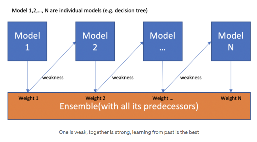
Boosting algorithm
We now understand that boosting combines a weak learner, a base learner to generate a strict rule. The first issue that should come to mind is, ‘How does boosting identify weak rules?’ We use machine learning (ML) techniques with a different distribution to uncover weak rules. Each time the base learning method is used, a new weak prediction rule is generated. This is a step-by-step procedure. After many rounds, the boosting approach combines numerous vulnerable laws into a single powerful prediction rule.
Gradient Boosting Classifier
This is one of the most powerful algorithms in machine learning. GB is a technique that is gaining popularity because of its high prediction speed and accuracy, mainly when dealing with big and complicated datasets as we know that the errors in machine learning algorithms are broadly classified into two categories, i.e. Bias Error and Variance Error. As gradient boosting is one of the boosting algorithms, it is used to minimize the bias error of the model.
Importance of Bias error
The biased degree to which a model’s prediction departs from the target value compared to the training data. Bias error occurs by reducing the assumptions employed in a model to approximate the target functions more efficiently. The model selection might induce bias.
Gradient Boosting – Working
It is based on the assumption that the best next model minimizes the total prediction error when merged with past models. The central concept is to define the desired outcomes for this next model to reduce error. How are the goals determined? The goal result for each instance in the data is determined by how much altering the forecast of that case affects the total prediction error,
Suppose a slight modification in a case’s prediction results in a substantial reduction in error; the case’s following target outcome is a high value. Predictions from the new model that is near to their objectives will help to decrease error.
If a slight adjustment in a case’s prediction results in no change in error, the case’s subsequent target outcome is zero. Changing this prediction does not affect the error.
Gradient boosting derives its name from the fact that goal outcomes for each instance are determined depending on the rise of the error about the forecast. In the space of feasible predictions for each training example, each new model takes a step toward minimizing prediction error.
Histogram based algorithm
A histogram is used to count or illustrate the frequency of data (number of occurrences) over discrete periods called bins. Each bin represents the frequency of the associated pixel value, and the histogram algorithm is conceptually quite simple.
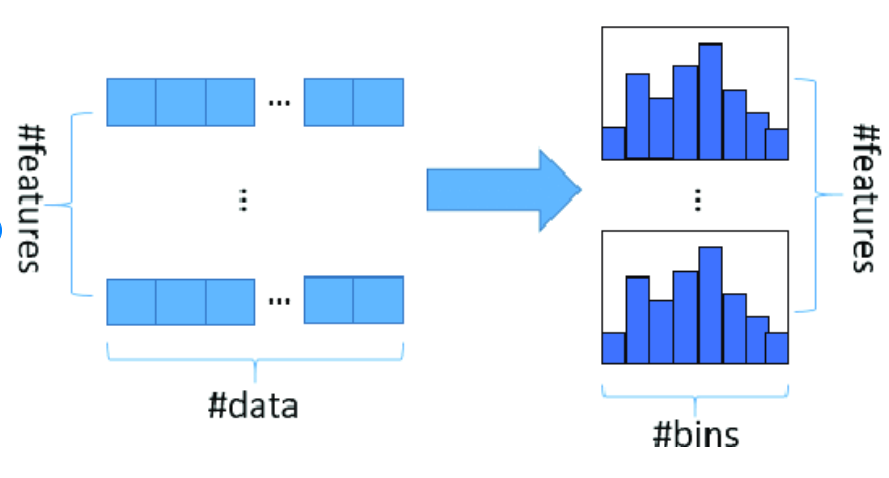
Histogram based Gradient Boosting
HGB will be available if we have scikit-learn v0.21.0 or a later version. In simple terms, we all know that binning is a concept used in data pre-processing, which means considering VIT university and dividing the students based on the state in our country like Tamilnadu, Kerala, Karnataka, and so on. After segmentation converts into numerical data, similarly, the same binning concept is applied to the Decision Tree (DT) algorithm. By reducing the number of features, it will be used to increase the algorithm’s speed. As a result, the same notion is employed in DT by grouping with histograms, which is known as the HGB classifier.
Parameters in Histogram based Gradient Boosting
In general, for all classifications, we have several parameters for fine-tuning our specific algorithms to achieve the best results. The same is true for the HBG classifier; while there are many factors, certain are critical, and those parameters about the HBG classifier are,
learning_rate, max_iter, max_depth, l2_regularization, each has some specific purpose of fine-tuning the model,
learning_rate deals with shrinkage, max_iter deals with the number of iterations needed for getting a good result, max_depth deals with several trees (Decision tree concepts), and l2_regularization, which deals with regularization concept to prevent overfitting problems.
Python Implementation of Histogram Boosting Gradient Classifier Classifier
#importing libraries
import numpy as np
import pandas as pd
import matplotlib.pyplot as plt
#importing datasets
normal = pd.read_csv('ptbdb_normal.csv')
abnormal = pd.read_csv('ptbdb_abnormal.csv')
#viewing normal dataset
normal.head()
#viewing abnormal dataset
abnormal.head()
#dimenion for normal
normal.shape
#dimension for abnormal
abnormal.shape
#changing the random column names to sequential - normal
#as we have some numbers name as columns we need to change that to numbers as
for normals in normal:
    normal.columns = list(range(len(normal.columns)))
#viewing edited columns for normal data
normal.head()
#changing the random column names to sequential - abnormal
#as we have some numbers name as columns we need to change that to numbers as
for abnormals in abnormal:
    abnormal.columns = list(range(len(abnormal.columns)))
#viewing edited columns for abnormal data
abnormal.head()
dataset.shape
#basic info of statistics
dataset.describe()
#basic information of dataset
dataset.info()
#missing values any from the dataset
print(str('Any missing data or NaN in the dataset:'), dataset.isnull().values.any())
#data ranges in the dataset - sample
print("The minimum and maximum values are {}, {}".format(np.min(dataset.iloc[-2,:].values), np.max(dataset.iloc[-2,:].values)))
#correlation for all features in the dataset
correlation_data =dataset.corr()
print(correlation_data)
import seaborn as sns
#visulaization for correlation
plt.figure(figsize=(10,7.5))
sns.heatmap(correlation_data, annot=True, cmap='BrBG')
#for target value count
label_dataset = dataset[187].value_counts()
label_dataset
#visualization for target label
label_dataset.plot.bar()
#splitting dataset to dependent and independent variable
X = dataset.iloc[:,:-1].values #independent values / features
y = dataset.iloc[:,-1].values #dependent values / target
#splitting the datasets for training and testing process
from sklearn.model_selection import train_test_split
X_train, X_test, y_train, y_test = train_test_split(X, y, test_size =0.3, random_state=42)
#size for the sets
print('size of X_train:', X_train.shape)
print('size of X_test:', X_test.shape)
print('size of y_train:', y_train.shape)
print('size of y_test:', y_test.shape)
#histogram boosting gradient classifer
from sklearn.experimental import enable_hist_gradient_boosting
from sklearn.ensemble import HistGradientBoostingClassifier
hgb_classifier = HistGradientBoostingClassifier()
hgb_classifier.fit(X_train,y_train)
y_pred_hgb = hgb_classifier.predict(X_test)
from sklearn.metrics import confusion_matrix, accuracy_score, roc_auc_score
cm_hgb = confusion_matrix(y_test, y_pred_hgb)
print(cm_hgb)
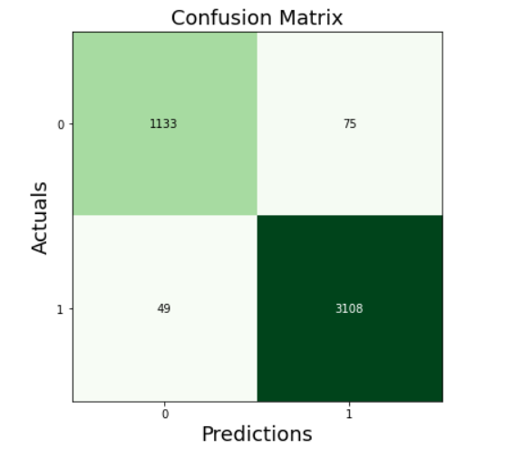
from mlxtend.plotting import plot_confusion_matrix
fig, ax = plot_confusion_matrix(conf_mat=cm_hgb, figsize=(6, 6), cmap=plt.cm.Greens)
plt.xlabel('Predictions', fontsize=18)
plt.ylabel('Actuals', fontsize=18)
plt.title('Confusion Matrix', fontsize=18)
plt.show()
from sklearn.model_selection import cross_val_score
accuracy_score(y_test, y_pred_hgb)
roc_auc_score(y_test, y_pred_hgb)
acc_hgb = cross_val_score(estimator = hgb_classifier, X = X_train, y = y_train, cv = 10)
print("Accuracy of hgb: {:.2f} %".format(acc_hgb.mean()*100))
print("SD of hgb: {:.2f} %".format(acc_hgb.std()*100))
print(metrics.classification_report(y_test, y_pred_hgb))
from sklearn.model_selection import GridSearchCV
parameters_hgb = [{'max_iter': [1000,1200,1500],
                'learning_rate': [0.1],
                'max_depth' : [25, 50, 75],
                'l2_regularization': [1.5],
                'scoring': ['f1_micro']}]
grid_search_hgb = GridSearchCV(estimator = hgb_classifier,
                           param_grid = parameters_hgb,
                           scoring = 'accuracy',
                           cv = 10,
                           n_jobs = -1)
grid_search_hgb.fit(X_train, y_train)
best_accuracy_hgb = grid_search_hgb.best_score_
best_paramaeter_hgb = grid_search_hgb.best_params_
print("Best Accuracy of HGB: {:.2f} %".format(best_accuracy_hgb.mean()*100))
print("Best Parameter of HGB:", best_paramaeter_hgb)

Accuracy score = 97.15%
Roc – Auc score = 0.9611
Accuracy (CV=10) = 97.56%
Grid Search Accuracy = 98.16%
https://github.com/anandprems/histogram_gradient_boosting_classifier, complete code can be accessed from this GitHub repository along with data description.
Conclusion
Hence, from this article, we can get some ideas about what machine learning is and its types, then classification type in supervised learning. Added we came across, why gradient algorithm and how it works and correlated with histogram concept to form histogram gradient boosting concept. I hope the python coding part clearly explains how much the Histogram Boosting Gradient Classifier algorithm helps in improving accuracy along with parameter fine-tuning.
Please leave your thoughts/opinions in the comments area below. Learning from your mistakes is my favourite quote; if you find something incorrect, highlight it; I am eager to learn from students like you.
About me, in short, I am Premanand. S, Assistant Professor Jr and a researcher in Machine Learning. I love to teach and love to learn new things in Data Science. Please mail me for any doubt or mistake, [email protected], and my LinkedIn https://www.linkedin.com/in/premsanand/.
The media shown in this article is not owned by Analytics Vidhya and are used at the Author’s discretion.


