Multi-label Text Classification Using Transfer Learning powered by “Optuna”

Tirthankar Das 22 Nov, 2022 • 7 min read

This article was published as a part of the Data Science Blogathon.

The problem of assigning more than one relevant label to the text is known as Multi-label Classification. Nowadays, Transfer learning is used as one of the most effective techniques to solve this problem. And we all face the challenges to decide optimum parameters at the classification step and trying our luck randomly. Here, “Optuna” comes into the picture.

Bhagawan Bharose Mat Baitho, Ka Pata Bhagawan Hamre Bharose Baith Ho!! (From the Movie: Manjhi-The Mountain Man)

Sorry, I just could not resist myself to refer to this quote as Optuna is passively telling us instead of following guts, it’s time to optimize (“Optuna”-mised) objective function.

Introduction

In this article, we are going to discuss fine-tuning of transfer learning-based Multi-label Text classification model using Optuna. It is an automatic hyperparameter optimization framework, particularly designed for Machine Learning & Deep Learning. The user of Optuna can dynamically construct the search spaces for the hyperparameters. The key features are in the following:

Lightweight, versatile, and Framework agnostic architecture
Efficient optimization algorithm
Easy parallelization
Quick visualization

Parameter optimization using Optuna can be done in the following three steps:

Wrap model training with an objective function and return accuracy/loss
Suggest hyper-parameters using a trial object
Create a study object and execute the optimization

Let’s do one project where we will build up a Multi-label Text Classification model using Transfer Learning. Here, we will tune the classification step using Optuna.

Fun Begins!!

Step1: Installation of packages
Step2: Data Collection
Step3: Sentence Embedding using the pre-trained model
Step4: Optuna based Hyper-Parameters tuning
Step5: Final Model Training and Prediction

Step 1 Installation of Packages

In this project, I am going to use the Kaggle kernel for model development. So, we need to install two important packages for this project i.e. sentence_transformers and Optuna. Before starting the installation, we need to make sure whether GPU is enabled.

sentence_transformers framework provides an easy method to compute dense vector representations for sentences, paragraphs, and images. The models are based on transformer networks like BERT / RoBERTa / XLM-RoBERTa etc. and achieve state-of-the-art performance in the various tasks.

!pip install sentence_transformers

Next, we need to install Optuna. It has the provision to use different samplers from Scikit-Optimize (skopt). Here, we need to create the study object and optimize it. What is great is that we can choose whether we want to maximize or minimize our objective function.

!pip install optuna

Once the above-mentioned two packages are installed, let’s import all the required packages and functions.

import numpy as np 
import pandas as pd
import random
import keras
import torch
import tensorflow as tf
import optuna
from optuna import Trial
from sklearn.model_selection import train_test_split
from sklearn.model_selection import KFold
from keras.callbacks import EarlyStopping,ReduceLROnPlateau
from sklearn.metrics import log_loss
from sentence_transformers import SentenceTransformer
import matplotlib.pyplot as plt
from sklearn import metrics
SEED = 99
def random_seed(SEED):
    random.seed(SEED)
    os.environ['PYTHONHASHSEED'] = str(SEED)
    np.random.seed(SEED)
    torch.manual_seed(SEED)
    torch.cuda.manual_seed(SEED)
    torch.cuda.manual_seed_all(SEED)
    torch.backends.cudnn.deterministic = True
    tf.random.set_seed(SEED)
random_seed(SEED)

Step 2 Data Collection

For this project, I will be going to use the dataset which has 6136 rows and 6 columns where the first column is the text field and the rest five columns are different labels.

train_data1 = pd.read_csv(‘train.csv’)
train_data1.head()

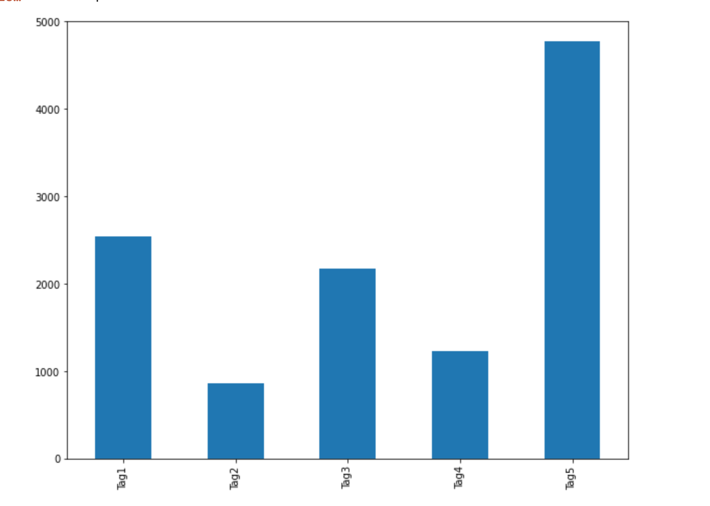
Let’s look at the distribution of different labels in our dataset.

comments_labels = train_data1[['Tag1','Tag2','Tag3','Tag4','Tag5']]
fig_size = plt.rcParams["figure.figsize"]
fig_size[0] = 10
fig_size[1] = 8
plt.rcParams["figure.figsize"] = fig_size
comments_labels.sum(axis=0).plot.bar()

Step 3 Sentence Embedding using the Pre-trained Model

Now, we will do text embedding using sentence_transformer. It provides state-of-the-art pre-trained models for more than 100 languages and is fine-tuned for various cases. For this project, we will be going to use bert-base-uncased model for embedding. As required, we can play around with other models too. Here, we also need to initialize the max_seq_length. It is set as 512 for this case.

model = SentenceTransformer('bert-base-uncased')
model.max_seq_length = 512
print("Max Sequence Length:", model.max_seq_length)
sentence_embeddings = model.encode(train_data1['Review'])

Once the sentence embedding is done, we will split the dataset into train and test. Then, the training dataset will be used for parameter optimisation. And, the test dataset will be used for validating model performance.

train1_x, test_x, train1_y, test_y = train_test_split(sentence_embeddings, 
                                                      comments_labels, 
                                                      train_size=0.8, 
                                                      test_size=0.2, 
                                                      random_state=42)

Step 4 Optuna based Hyper-Parameters Tunning

So, we have reached the most interesting and complex part of this project. Now, I am going to use Neural Network to solve this Multi-label text classification model. When we build the NN model, various questions come into mind such as what should be the ideal number of hidden layers and hidden nodes, optimum dropout value, optimum batch size, ideal activation function, etc. These are nothing but Hyperparameters. A Hyperparameter is a parameter that is set before the learning process begins. These parameters are tunable and can directly affect how well the model trains. In order to achieve maximal performance, it is important to understand how to optimize them. Ther are some common strategies for optimizing Hyperparameters:

Grid Search: Search a set of manually predefined hyperparameters
Random Search: Similar to grid search, but replaces the exhaustive search with random search
Bayesian Optimization: Builds a probabilistic model of the function mapping to evaluate test data
Gradient-Based Optimization: Compute gradient using hyperparameters and then optimize it

Today’s deep learning algorithms often contain many hyperparameters, and it takes days, weeks to train a good model. It is simply not possible to brute force сombinations of hyperparameters and train separate models for each without any optimizations. That’s why we need a Hyperparameter optimiser.

Optuna combines sampling and pruning mechanisms to provide efficient hyperparameter optimization. The pruning mechanism implemented in Optuna is based on an asynchronous variant of the Successive Halving Algorithm (SHA) and Tree-structured Parzen Estimator (TPE) is the default sampler in Optuna.

There are no other packages that can optimize Chainer Hyperparameters better than Optuna. In the vector space, it supports all three types of data i.e. Integer, Float, and Categorical. Now let’s have a close look into the steps of Optuna.

Here, we have created an objective function that will try to minimize the validation loss. Hyperparameters are suggested using the ‘trial’ object. We are optimizing the following hyperparameters:

Number of Hidden Layers: [1,2,3]
Number of Hidden Nodes inside the Hidden layers: [48 : len(sentence_embeddings[0])]
Activation Function: [‘relu’, ‘linear’,’swish’]
Dropout Rate: [0:0.6]
Batch Size:[8:128]

It can be further expanded and adopted for other parameters also.

def objective(trial):
    keras.backend.clear_session()
    train_x, valid_x, train_y, valid_y = train_test_split(train1_x, train1_y, train_size=0.8, test_size=0.2,
                                                                random_state=42)
    #optimum number of hidden layers
    n_layers = trial.suggest_int('n_layers', 1, 3)
    model = keras.Sequential()
    for i in range(n_layers):
        #optimum number of hidden nodes
        num_hidden = trial.suggest_int(f'n_units_l{i}', 48, len(sentence_embeddings[0]), log=True)
        #optimum activation function
        model.add(keras.layers.Dense(num_hidden, input_shape=(len(sentence_embeddings[0]),),
                               activation=trial.suggest_categorical(f'activation{i}', ['relu', 'linear','swish'])))
        #optimum dropout value
        model.add(keras.layers.Dropout(rate = trial.suggest_float(f'dropout{i}', 0.0, 0.6)))

    model.add(keras.layers.Dense(5,activation=tf.keras.activations.sigmoid)) #output Layer
    val_ds = (valid_x,valid_y)
    reduce_lr = ReduceLROnPlateau(monitor='val_loss', factor=0.1,patience=1,min_lr=1e-05,verbose=0)
    early_stoping = EarlyStopping(monitor="val_loss",min_delta=0,patience=5,verbose=0,mode="auto", baseline=None,restore_best_weights=True)
    model.compile(loss='binary_crossentropy',metrics='categorical_crossentropy', optimizer='Adam')
    #optimum batch size
    histroy = model.fit(train_x,train_y, validation_data=val_ds,epochs=200,callbacks=[reduce_lr,early_stoping],verbose=0,
                       batch_size=trial.suggest_int('size', 8, 128))
    return min(histroy.history['val_loss'])

The next step is to create a Study object and execute the optimization steps. Once it is done, we need to find out the best parameter settings from the Study object. Here, we have set the threshold on both Maximum Trials (n_trial) and Maximum Time(timeout).

if __name__ == "__main__":
  study = optuna.create_study(direction="minimize")
  study.optimize(objective, n_trials=50, timeout=1200)
  print("Number of finished trials: {}".format(len(study.trials)))
  print("Best trial:")
  trial = study.best_trial
  print("  Value: {}".format(trial.value))

Once the optimization step is executed completely, we will look at the best trial. It can be visualised using the following code also:

optuna.visualization.plot_optimization_history(study)

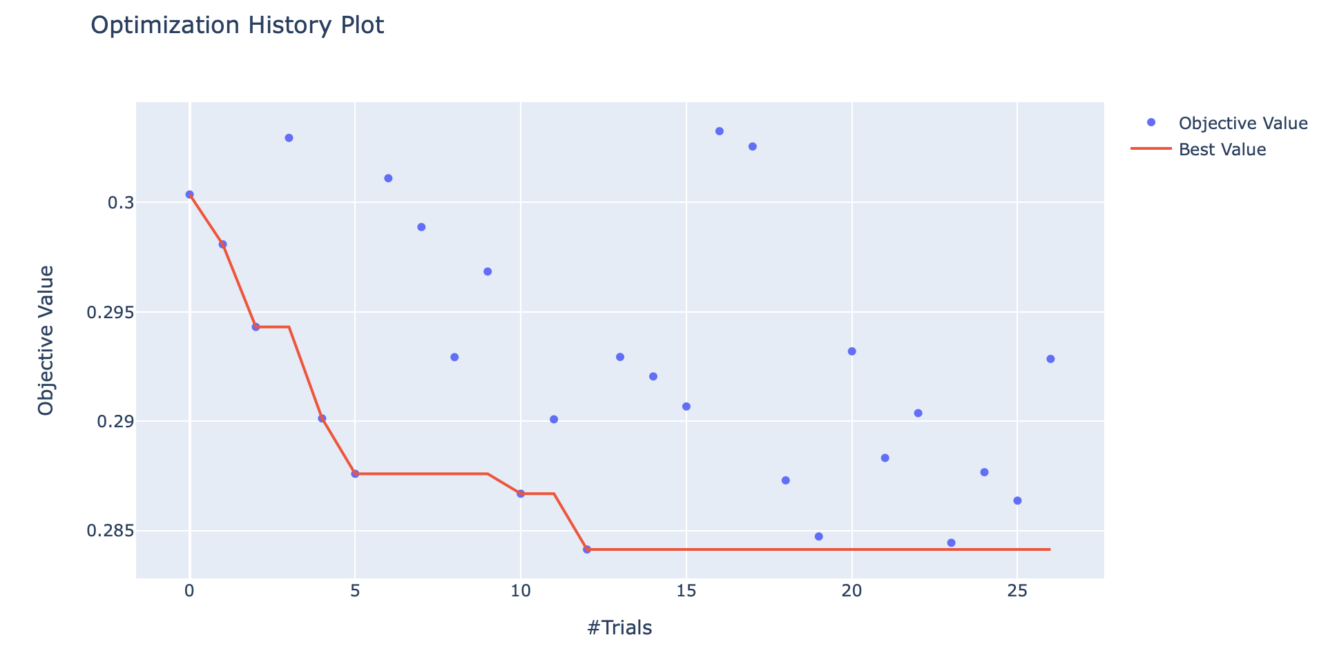
From the plot we can clearly understand that the 12th trial was best as it has a minimum loss value and corresponding optimum hyperparameters can be found using the following code:

print("  Params: ")
for key, value in trial.params.items():
  print("    {}: {}".format(key, value))

The output looks like this:

Params: 
    n_layers: 1
    n_units_l0: 682
    activation0: relu
    dropout0: 0.42199525694641216
    size: 34

Step 5 Final Model Training and Prediction

Now, we will utilize the optimum parameters to create the final model and use it for final training. Now, find the final model in the following:

def wider_model():
    model = keras.Sequential()
    model.add(keras.layers.Dense(682,input_shape=(len(sentence_embeddings[0]),),activation=tf.keras.activations.relu))
    model.add(keras.layers.Dropout(0.42199525694641216))
    model.add(keras.layers.Dense(5,activation=tf.keras.activations.sigmoid))
    return model

I am trying out 5 Fold Cross-validation method for predicting test dataset based on the following code:

skf = KFold(n_splits=5, shuffle=True, random_state=1234)
Final_Subbmission = []
val_loss_print = []
i=1
for train_index, test_index in skf.split(train1_x,train1_y):
    keras.backend.clear_session()
    print('#################')
    print(i)
    print('#################')
    X_train, X_test = train1_x[train_index], train1_x[test_index]
    y_train, y_test = train1_y.iloc[train_index], train1_y.iloc[test_index]
    model = wider_model()
    val_ds = (X_test,y_test)
    reduce_lr = ReduceLROnPlateau(monitor='val_loss', factor=0.1,patience=1,min_lr=1e-05,verbose=1)
    early_stoping = EarlyStopping(monitor="val_loss",min_delta=0,patience=5,verbose=1,mode="auto", baseline=None,restore_best_weights=True)
    model.compile(loss='binary_crossentropy',metrics='categorical_crossentropy', optimizer='Adam')
    histroy = model.fit(X_train,y_train, validation_data=val_ds,epochs=200,callbacks=[reduce_lr,early_stoping],verbose=1,batch_size=34)
    print(min(histroy.history['val_loss']))
    val_loss_print.append(min(histroy.history['val_loss']))
    Test_seq_pred = model.predict(test_x)
    Final_Subbmission.append(Test_seq_pred)
    i=i+1

This cross-validation method will generate 5 different sets of probability for each class of the Test dataset. Now, we will take the mean of these probabilities.

Test_prob =np.mean(Final_Subbmission,0)
Test_prob = pd.DataFrame(Test_prob)
Test_prob.columns = comments_labels.columns

In Multi-label classification, we can use Mean Average Precision to measure the model performance. Let’s check the value for our test dataset.

test_y1 = test_y.reset_index(drop=True)
print("weighted: {:.2f} ".format( metrics.average_precision_score(test_y1, Test_prob, average='weighted')))

The output looks like this:

weighted: 0.90

So, we are able to achieve 0.9 MAP with the help of the Optuna hyperparameter tuner. If you are not yet convinced or want to improve the model further, please go through Optuna Home page and empower yourself.

Conclusion

In this article, I have explained three magic steps to develop a very effective Multi-label Text classification model i.e firstly Sentence Embedding using sentence_transformers, next Optuna based hyperparameter optimisation for Neural Network model and finally Train the model with an optimum set of hyperparameters.

Though, I have explained the application of Optuna for Multi-label Text classification. But this can be further adapted to other Regression or Classification models also. We can judiciously apply Optuna for all kinds of structured/unstructured datasets. We can use it for PyTorch, TensorFlow, keras, XGboost, LightGBM, Scikit-Learn, MXNet etc. More Power to Data Scientist!!

Happy Learning!!

Reference

Your suggestions and doubts are welcomed here in the comment sections. Thank you for reading my article.

About the author

Tirthankar Das: Data Science professional with 7.5 years experience in different domains such as Banking & Finance, Aviation, Manufacturing, and Pharmaceuticals. Happy to connect over LinkedIn

The media shown in this article is not owned by Analytics Vidhya and are used at the Author’s discretion.

Tirthankar Das 22 Nov 2022

Advanced NLP Python Text Word Embeddings