The Complete LSTM Tutorial With Implementation
This article was published as a part of the Data Science Blogathon.
Introduction
Artificial Neural Networks (ANN) have paved a new path to the emerging AI industry since decades it has been introduced. With no doubt in its massive performance and architectures proposed over the decades, traditional machine-learning algorithms are on the verge of extinction with deep neural networks, in many real-world AI cases.
But, every new invention in technology must come with a drawback, otherwise, scientists cannot strive and discover something better to compensate for the previous drawbacks. Similarly, Neural Networks also came up with some loopholes that called for the invention of recurrent neural networks.
Why Recurrent?
In Neural Networks, we stack up various layers, composed of nodes that contain hidden layers, which are for learning and a dense layer for generating output. But, the central loophole in neural networks is that it does not have memory. Since no memory is associated, it becomes very difficult to work on sequential data like text corpora where we have sentences associated with each other, and even time-series where data is entirely sequential and dynamic.
Here, Recurrent Neural Networks comes to play. RNN addresses the memory issue by giving a feedback mechanism that looks back to the previous output and serves as a kind of memory. Since the previous outputs gained during training leaves a footprint, it is very easy for the model to predict the future tokens (outputs) with help of previous ones.
Why LSTM when we have RNN?
A sentence or phrase only holds meaning when every word in it is associated with its previous word and the next one. LSTM, short for Long Short Term Memory, as opposed to RNN, extends it by creating both short-term and long-term memory components to efficiently study and learn sequential data. Hence, it’s great for Machine Translation, Speech Recognition, time-series analysis, etc.
Tutorial Overview
In this tutorial, we will have an in-depth intuition about LSTM as well as see how it works with implementation!
Let’s have a look at what we will cover-
- A Quick Look into LSTM Architecture
- Why does LSTM outperform RNN?
- Deep Learning about LSTM gates
- An Implementation is Necessary!
- Wrap Up with Bonus Resources
So, let’s dive into the LSTM tutorial!
A Quick Look into LSTM Architecture
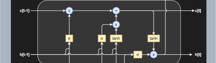
Let’s see how a simple LSTM black box model looks-
Source -MachineCurve
To give a gentle introduction, LSTMs are nothing but a stack of neural networks composed of linear layers composed of weights and biases, just like any other standard neural network. The weights are constantly updated by backpropagation.
Now, before going in-depth, let me introduce a few crucial LSTM specific terms to you-
- Cell — Every unit of the LSTM network is known as a “cell”. Each cell is composed of 3 inputs —
- x(t) — token at timestamp t
- h(t−1) — previous hidden state
- c(t-1) — previous cell state,
and 2 outputs —
- h(t) — updated hidden state, used for predicting the output
- c(t) — current cell state
2. Gates — LSTM uses a special theory of controlling the memorizing process. Popularly referred to as gating mechanism in LSTM, what the gates in LSTM do is, store the memory components in analog format, and make it a probabilistic score by doing point-wise multiplication using sigmoid activation function, which stores it in the range of 0–1. Gates in LSTM regulate the flow of information in and out of the LSTM cells.
Gates are of 3 types —
- Input Gate — This gate lets in optional information necessary from the current cell state. It decides which information is relevant for the current input and allows it in.
- Output Gate — This gate updates and finalizes the next hidden state. Since the hidden state contains critical information about previous cell inputs, it decides for the last time which information it should carry for providing the output.
- Forget Gate — Pretty smart in eliminating unnecessary information, the forget gate multiplies 0 to the tokens which are not important or relevant and lets it be forgotten forever.
Why does LSTM outperform RNN?
First, let’s take a comparative look into an RNN and an LSTM-
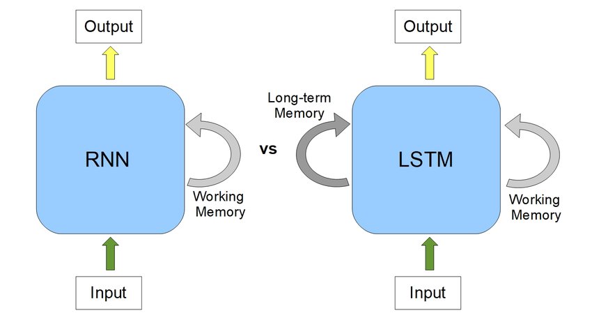
RNNs have quite massively proved their incredible performance in sequence learning. But, it has been remarkably noticed that RNNs are not sporty while handling long-term dependencies.
Why so?
Vanishing Gradient Problem
Recurrent Neural Networks uses a hyperbolic tangent function, what we call the tanh function. The range of this activation function lies between [-1,1], with its derivative ranging from [0,1]. Now we know that RNNs are a deep sequential neural network. Hence, due to its depth, the matrix multiplications continually increase in the network as the input sequence keeps on increasing. Hence, while we use the chain rule of differentiation during calculating backpropagation, the network keeps on multiplying the numbers with small numbers. And guess what happens when you keep on multiplying a number with negative values with itself? It becomes exponentially smaller, squeezing the final gradient to almost 0, hence weights are no more updated, and model training halts. It leads to poor learning, which we say as “cannot handle long term dependencies” when we speak about RNNs.
Exploding Gradient Problem
Similar concept to the vanishing gradient problem, but just the opposite of the process, let’s suppose in this case our gradient value is greater than 1 and multiplying a large number to itself makes it exponentially larger leading to the explosion of the gradient.
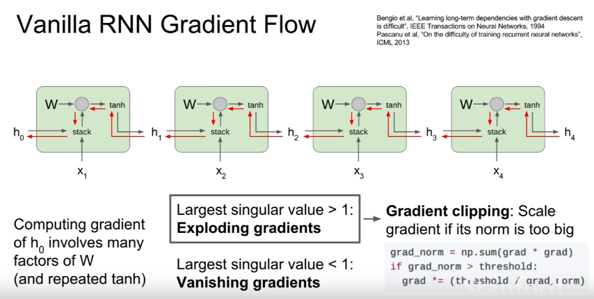
Source – Stanford NLP
This also leads to the major issue of Long Term Dependency.
Long Term Dependency Issue in RNNs
Let us consider a sentence-
“I am a data science student and I love machine ______.”
We know the blank has to be filled with ‘learning’. But had there been many terms after “I am a data science student” like, “I am a data science student pursuing MS from University of…… and I love machine ______”.
This time, however, RNNS fails to work. Likely in this case we do not need unnecessary information like “pursuing MS from University of……”. What LSTMs do is, leverage their forget gate to eliminate the unnecessary information, which helps them handle long-term dependencies.
Deep Learning about LSTM gates
Let’s learn about LSTM gates in-depth.
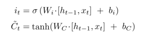
The Input Gate
As discussed earlier, the input gate optionally permits information that is relevant from the current cell state. It is the gate that determines which information is necessary for the current input and which isn’t by using the sigmoid activation function. It then stores the information in the current cell state. Next, comes to play the tanh activation mechanism, which computes the vector representations of the input-gate values, which are added to the cell state.
Source – Stanford NLP
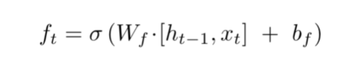
The Forget Gate
We already discussed, while introducing gates, that the hidden state is responsible for predicting outputs. The output generated from the hidden state at (t-1) timestamp is h(t-1). After the forget gate receives the input x(t) and output from h(t-1), it performs a pointwise multiplication with its weight matrix with an add-on of sigmoid activation which generates probability scores. These probability scores help it determine what is useful information and what is irrelevant.
Source – Stanford NLP
Cell State Update Mechanism
Replacing the new cell state with whatever we had previously is not an LSTM thing! An LSTM, as opposed to an RNN, is clever enough to know that replacing the old cell state with new would lead to loss of crucial information required to predict the output sequence.
That’s where LSTM beats RNN, remember?!
By now, the input gate remembers which tokens are relevant and adds them to the current cell state with tanh activation enabled. Also, the forget gate output, when multiplied with the previous cell state C(t-1), discards the irrelevant information. Hence, combining these two gates’ jobs, our cell state is updated without any loss of relevant information or the addition of irrelevant ones.
.png)
Output Gate
This gate, which pretty much clarifies from its name that it is about to give us the output, does a quite straightforward job. The output gate decides what to output from our current cell state. The output gate, also has a matrix where weights are stored and updated by backpropagation. This weight matrix, takes in the input token x(t) and the output from previously hidden state h(t-1) and does the same old pointwise multiplication task. However, as said earlier, this takes place on top of a sigmoid activation as we need probability scores to determine what will be the output sequence.
After we get the sigmoid scores, we simply multiply it with the updated cell-state, which contains some relevant information required for the final output prediction. A final tanh multiplication is applied at the very last, to ensure the values range from [-1,1], and our output sequence is ready!
.png)
An Implementation is Necessary!
Step 1: Import the dependencies and code the activation functions-
import random
import numpy as np
import math
def sigmoid(x):
    return 1. / (1 + np.exp(-x))
def sigmoid_derivative(values):
    return values*(1-values)
def tanh_derivative(values):
    return 1. - values ** 2
# createst uniform random array w/ values in [a,b) and shape args
def rand_arr(a, b, *args):
    np.random.seed(0)
    return np.random.rand(*args) * (b - a) + a
Step 2: Initializing the biases and weight matrices
class LstmParam:
    def __init__(self, mem_cell_ct, x_dim):
        self.mem_cell_ct = mem_cell_ct
        self.x_dim = x_dim
        concat_len = x_dim + mem_cell_ct
        # weight matrices
        self.wg = rand_arr(-0.1, 0.1, mem_cell_ct, concat_len)
        self.wi = rand_arr(-0.1, 0.1, mem_cell_ct, concat_len)
        self.wf = rand_arr(-0.1, 0.1, mem_cell_ct, concat_len)
        self.wo = rand_arr(-0.1, 0.1, mem_cell_ct, concat_len)
        # bias terms
        self.bg = rand_arr(-0.1, 0.1, mem_cell_ct)
        self.bi = rand_arr(-0.1, 0.1, mem_cell_ct)
        self.bf = rand_arr(-0.1, 0.1, mem_cell_ct)
        self.bo = rand_arr(-0.1, 0.1, mem_cell_ct)
        # diffs (derivative of loss function w.r.t. all parameters)
        self.wg_diff = np.zeros((mem_cell_ct, concat_len))
        self.wi_diff = np.zeros((mem_cell_ct, concat_len))
        self.wf_diff = np.zeros((mem_cell_ct, concat_len))
        self.wo_diff = np.zeros((mem_cell_ct, concat_len))
        self.bg_diff = np.zeros(mem_cell_ct)
        self.bi_diff = np.zeros(mem_cell_ct)
        self.bf_diff = np.zeros(mem_cell_ct)
        self.bo_diff = np.zeros(mem_cell_ct)
Step 3: Multiplying forget gate with last cell state to forget irrelevant tokens
#stacking x(present input xt) and h(t-1)
xc = np.hstack((x,  h_prev))
#dot product of Wf(forget weight matrix and xc +bias)
self.state.f = sigmoid(np.dot(self.param.wf, xc) + self.param.bf)
#finally multiplying forget_gate(self.state.f) with previous cell state(s_prev)
#to get present state.
self.state.s = self.state.g * self.state.i + s_prev * self.state.f
Step 4: Sigmoid Activation decides which values to take in and tanh transforms new tokens to vectors
#xc already calculated above
self.state.i = sigmoid(np.dot(self.param.wi, xc) + self.param.bi)
#C(t)
self.state.g = np.tanh(np.dot(self.param.wg, xc) + self.param.bg)
Step 5: Calculate the present cell state
#to calculate the present state
self.state.s = self.state.g * self.state.i + s_prev * self.state.f
Step 6: Calculate the output state
#to calculate the output state
self.state.o = sigmoid(np.dot(self.param.wo, xc) + self.param.bo)
#output state h
self.state.h = self.state.s * self.state.o
So, this is how a single node of LSTM works! You can check the entire implementation here.
Wrap Up with Bonus Resources
Hope you have clearly understood how LSTM works and why is it better than RNN! If you are still curious and want to explore more, you can check on these awesome resources –
1. Colah’s Blog
Conclusion
Long Short Term Memories are very efficient for solving use cases that involve lengthy textual data. It can range from speech synthesis, speech recognition to machine translation and text summarization. I suggest you solve these use-cases with LSTMs before jumping into more complex architectures like Attention Models.
Read more articles on LSTM.
If you liked this article, feel free to share it with your network😄. For more articles about Data Science and AI, follow me on Medium and LinkedIn.
Happy Machine Learning.
The media shown in this article is not owned by Analytics Vidhya and are used at the Author’s discretion.


