A Comprehensive Guide on ggplot2 in R
This article was published as a part of the Data Science Blogathon.
.jpg)
Image source: Author
Introduction
Visualization plays a pivotal role in the decision-making process after analyzing relevant data. Graphical representation, such as the use of the ggplot2 library in R, highlights the interdependence of key elements affecting performance. In addition to ggplot2, there are many other libraries in Python and R that provide diverse options for creating various geometrical and pictorial visualizations. These visualizations not only have the potential to be aesthetically attractive but also convey valuable and informative insights
R supports a variety of functions and data visualization packages to build interactive visuals for exploratory data analysis. One such library available in R is ggplot2. This guide will focus on the visualization capabilities of ggplot2 in R. You will learn to create some popular plots and customize them using the ggplot2 in R.
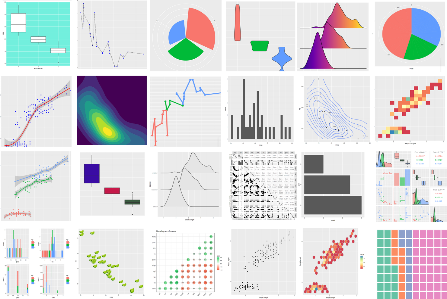
Image source: Author
Table of contents
What is ggplot and it latest version ggplot2?
ggplot2 is a popular data visualization package in the R programming language. It was developed by Hadley Wickham and is based on the principles of the “Grammar of Graphics,” which provides a systematic and structured approach to creating and understanding data visualizations. ggplot2 allows users to create a wide variety of high-quality and customizable statistical graphs, making it a valuable tool for data exploration and presentation.
ggplot2 in R is the latest version of the famous open-source data visualization tool ggplot for the statistical programming language R. The term ggplot2 relates to the package’s name. We use the function ggplot() to produce the plots when using the package. Therefore, ggplot() is the command, and the whole package is called ggplot2. It is a part of the R tidyverse, an ecosystem of packages designed with common APIs.
It is the most widely used alternative to base R graphics. It is based on the Grammar of Graphics and is highly flexible. It allows us to build and customize graphics by adding more layers. This library makes it simple to create ready-to-publish charts. The ggplot2 in R package includes themes for personalizing charts. With the theme function components, the colours, line types, typefaces, and alignment of the plot can be changed, among other things. Various options allow you to personalize the graph by adding titles, subtitles, arrows, texts, or lines.
The Grammar of Graphics helps us build graphical representations from different visual elements. This grammar allows us to communicate about plot components. The Grammar of Graphics was created by Leland Wilkinson and was adapted by Hadley Wickham.
A ggplot is made up of a few basic components:
Data: The raw data that you want to plot.
Geometries geom_: The geometric shapes used to visualize the data.
Aesthetics aes(): Aesthetics pertaining to the geometric and statistical objects, like colour, size, shape, location, and transparency
Scales scale_: includes a set of values for each aesthetic mapping in the plot
Statistical transformations stat_: calculates the different data values used in the plot.
Coordinate system coord_: used to organize the geometric objects by mapping data coordinates
Facets facet_: a grid of plots is displayed for groups of data.
Visual themes theme(): The overall visual elements of a plot, like grids & axes, background, fonts, and colours.
Prerequisites are R and R Studio before installing ggplot2. Alternatively, you may go for Kaggle or Google Colab for ggplot2.
Installing ggplot2
So let us begin by first installing this package using the R function ‘install. packages()’.
install.packages('ggplot2')It’s important to note that ggplot2 comes with multiple pre-installed data sets. To see the entire list of pre-installed datasets, run the following command:
data()This guide will use the ‘Iris’ dataset and ‘Motor trend car road tests’ dataset.
The iris dataset contains dimensions for 50 flowers from three distinct species on four different features (in centimetres). We can import the iris dataset using the following command because it is a built-in dataset in R:
data(iris)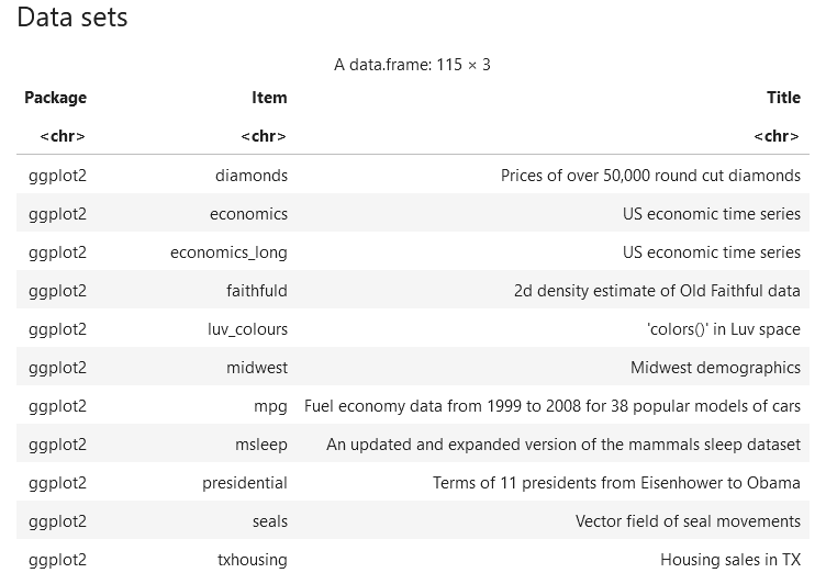
The dim function can be used to display the rows and columns of the dataset.
dim(iris)The iris dataset contains 150 rows and 5 columns. Using the head() function, we can explore the first few rows of the dataset.
head(iris)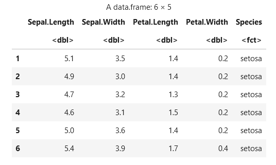
If you wish to quickly summarize the dataset, use the summary() function and it will summarize each variable in the dataset.
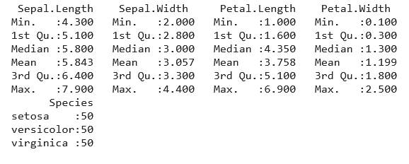
For all the numeric variables in the dataset, we get the following information:
Min: The minimum value of the variable.
1st Qu: 25th percentile or first quartile.
Median: Central value.
Mean: Average value.
3rd Qu: 75th percentile or third quartile.
Max: Maximum value.
For the categorical variable in the dataset, we get the frequency count of each value:
setosa: This type of species has 50 values.
versicolor: This type of species has 50 values.
virginica: This type of species has 50 values.
The ggplot2 is made of three basic elements: Plot = Data + Aesthetics + Geometry.
Following are the essential elements of any plot:
Data: It is the dataframe.
Aesthetics: It is used to represent x and y in a graph. It can alter the colour, size, dots, the height of bars etc.
Geometry: It defines the graphics type, i.e., scatter plot, bar plot, jitter plot etc.
Scatter Plot
Now we will start this tutorial with a scatter plot. To plot it, we will be using the geom_point() function. Here we will plot the Sepal length variable on the x-axis and the petal length variable on the y axis.
ggplot(iris, aes(x=Sepal.Length, y=Petal.Length))+geom_point()It’s important to note that you use the addition (+) operator to add the geom layer. You’ll always use the (+) operator when you increase the number of layers in your visualization.
The dataset contains a number of species. It will be interesting to see how the length of the sepals and petals changes between species. It’s only a matter of applying a colour parameter to the aesthetics. We will set the colour to species. As a result, the different species can be visualized by different colours.
ggplot(iris, aes(x=Sepal.Length, y=Petal.Length, col=Species))+geom_point()
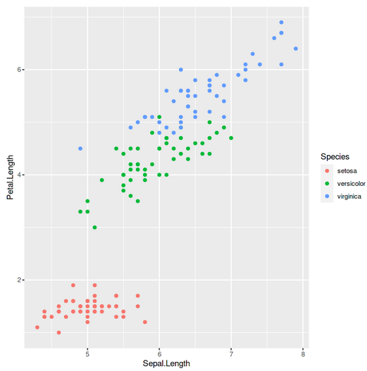
Note that colour, colour and col are all supported by ggplot2.
Aesthetic mappings utilize data characteristics to alter visual features like colour, size, shape, or transparency. As a result, each feature adds an element of the data and be used to transmit information. The aes() method specifies all aesthetics for a plot.
We can plot different shapes for different species by using the following command:
ggplot(iris, aes(x=Sepal.Length, y=Petal.Length, col=Species, shape=Species))+geom_point()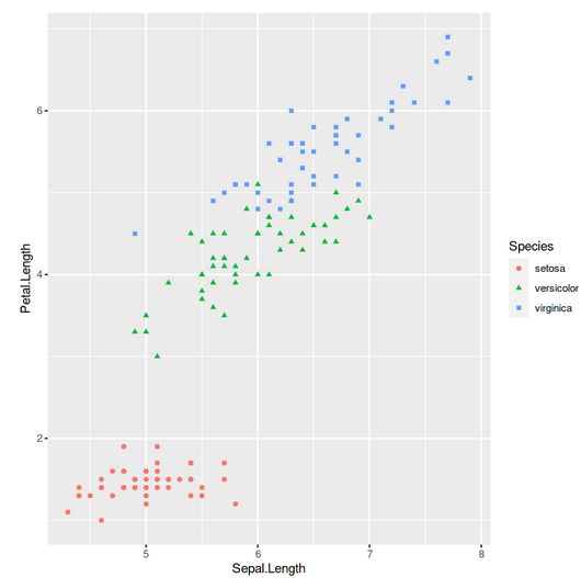
ggplot2 may be used to create different types of plots based on these fundamentals. These graphs are created using functions from the Grammar of Graphics. The difference between plots is the number of geometric objects (geoms) they contain. Geoms are supported by ggplot2 in a variety of ways for plotting different graphs like:
- Scatter Plot: To plot individual points, use geom_point
- Bar Charts: For drawing bars, use geom_bar
- Histograms: For drawing binned values, geom_histogram
- Line Charts: To plot lines, use geom_line
- Polygons: To draw arbitrary shapes, use geom_polygon
- Creating Maps: Use geom_map for drawing polygons in the shape of a map by using the map_data() function
- Creating Patterns: Use the geom_smooth function for showing simple trends or approximations
A variety of geometries can be added to a plot, allowing you to build complex visualizations that display multiple elements of your data.
ggplot(iris, aes(x=Sepal.Length, y=Petal.Length, col=Species))+geom_point() +geom_smooth()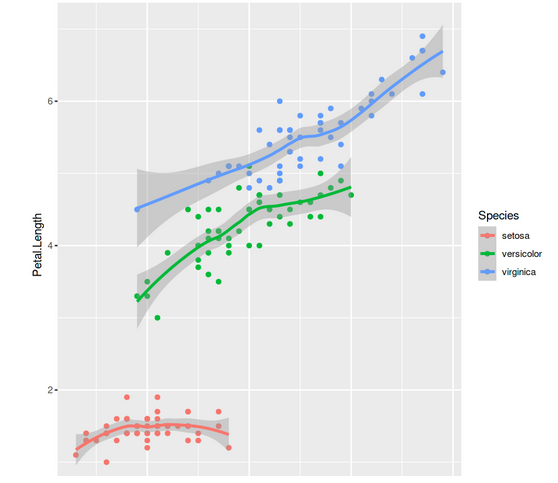
Points and smoothed lines can be plotted together for the same x and y variables, but with different colours for each geom.
ggplot(iris, aes(x=Sepal.Length, y=Petal.Length, col=Species))
       +geom_point(color = "blue") + geom_smooth(color = "red")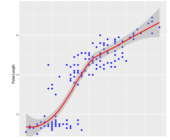
If the ggplot includes an aesthetic, it will be passed on to each consecutive geom point. Alternatively, we can define certain aes inside each geom, just displaying certain features for it.
# color aesthetic defined for each geom point
ggplot(iris, aes(x=Sepal.Length, y=Petal.Length, col=Species))
       +geom_point() +geom_smooth(se = FALSE)
# color aesthetic defined only for a particular geom_point layer
ggplot(iris, aes(x=Sepal.Length, y=Petal.Length)) +geom_point(aes(col = Species))
+geom_smooth(se = FALSE)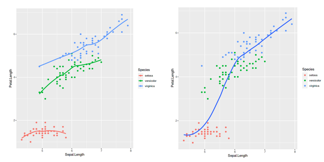
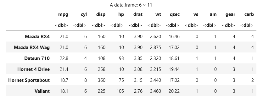
Now we will use ‘mtcars’ dataset, i.e., the ‘Motor Trend Car Road Tests’ dataset from the pre-installed data sets for our next visualizations. We will import the dataset using the data() command and get a glimpse of the dataset using the glimpse() command, respectively. Note you have to install and import the tidyverse package here; otherwise, it will throw an error.
data(mtcars)
library (tidyverse)
glimpse (mtcars)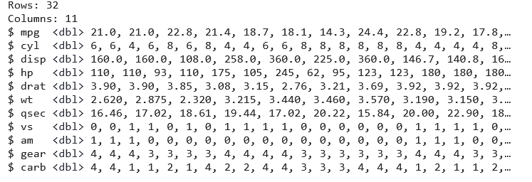
As we can see, the dataset contains 32 observations of 11 variables. This dataset is small, simple, and consists of continuous and categorical variables. The columns of the mtcars dataset are:
- mpg – Miles/(US) gallon
- cyl – Number of cylinders (4, 6, 8)
- disp – Displacement (cu.in.)
- hp – Gross horsepower
- drat – Rear axle ratio
- wt – Weight (1000 lbs)
- qsec – 1/4 mile time
- vs – V/S (0, 1)
- am – Transmission (0 = automatic, 1 = manual)
- gear – Number of forward gears (3, 4, 5)
- carb – Number of carburetors (1, 2, 3, 4, 6, 8)
Bar Plot
This plot is used to measure changes over a particular span of time. It is the best option to represent the data when changes are large.
First, we will plot the bar chart for this dataset using the following command:
ggplot(mtcars, aes(x = gear)) +geom_bar()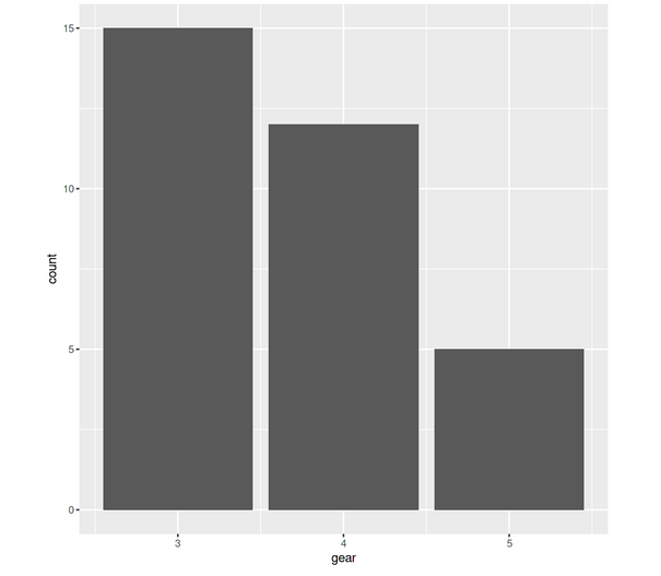
Using the coord_flip() command, you can interchange the x-axis and y-axis,
ggplot(mtcars, aes(x = gear)) +geom_bar()+coord_flip()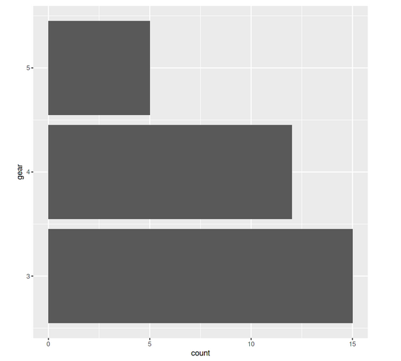
Statistical Transformations
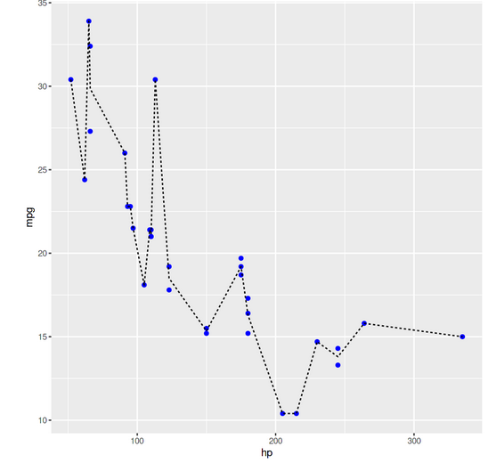
Many different statistical transformations are supported by ggplot2. For more levels, we can directly call stat_ functions. For example, here, we make a scatter plot of horsepower vs mpg and then use stat summary to draw the mean.
ggplot(mtcars, aes(hp, mpg)) + geom_point(color = "blue")
       + stat_summary(fun.y = "mean", geom = "line", linetype = "dashed")
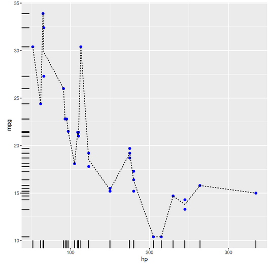
A rug displays the data of a single quantitative parameter on the axis in the form of markings. It is often used in conjunction with scatter plots or heatmaps to illustrate the overall distribution of one or both variables.
ggplot(mtcars, aes(hp, mpg)) + geom_point(color = "blue")
       + geom_rug(show.legend = FALSE) +stat_summary(fun.y = "mean",
         geom = "line", linetype = "dashed")
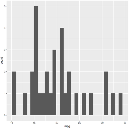
Histogram
A Histogram is used to show the frequency distribution of a continuous-discrete variable.
Using the geom_histogram() command, we can create a simple histogram:
ggplot(mtcars,aes(x=mpg)) + geom_histogram()
Box Plot
A Box plot displays the distribution of the data and skewness in the data with the help of quartile and averages.
Similarly, we can use the geom_boxplot() command for plotting a box plot. We will plot mpg vs cyl. Before plotting the box plot, we will visualize the first few rows by running the head() command:
As we can see from the image, mpg is a continuous variable, while cyl is categorical. So before plotting, we convert the variable cyl to a factor. Below is the output graph.
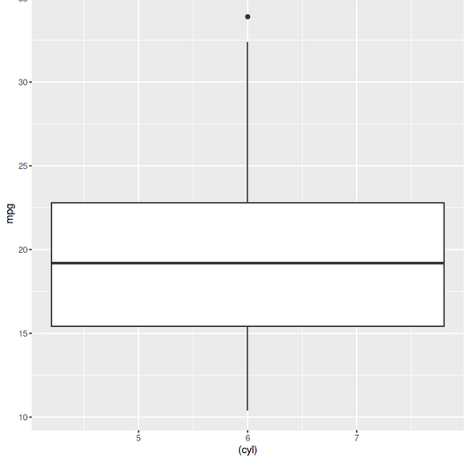
So, we will use the following command to plot the graph:
ggplot(mtcars, aes(x=as.factor(cyl), y=mpg)) + geom_boxplot()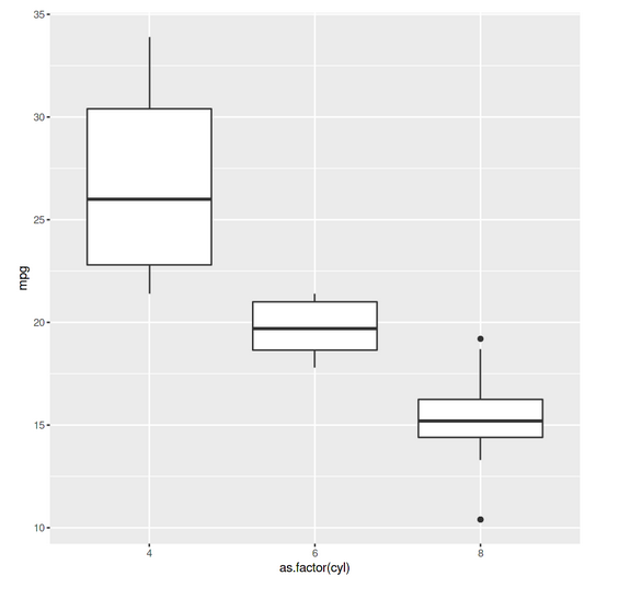
If we want to change the boundary colour of the boxplot, we have to use the scale_color_manual() function with the hex values of colours of our choice.
mtcars$cyl <- as.factor(mtcars$cyl)
ggplot(mtcars, aes(x=(cyl), y=mpg,color = cyl)) + geom_boxplot()
       +scale_color_manual(values = c("#3a0ca3", "#c9184a", "#3a5a40"))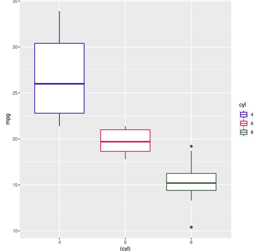
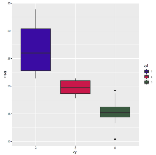
Alternatively, we can use the same logic to fill the colour in the box plot instead of just changing the colour of the outline:
Violin Plot
This plot is used to plot the numeric data, which is similar to a box plot and kernel density plot combination. It can show data peaks and distribution of the data.
ggplot(mtcars, aes(factor(cyl), mpg))+ geom_violin(aes(fill = cyl))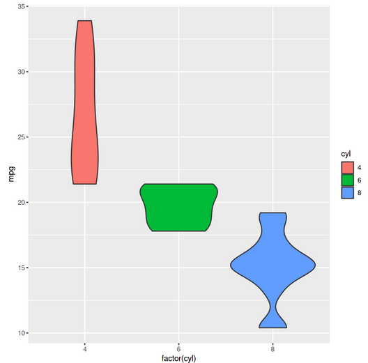
Pie Chart
The pie chart shows the proportions as a part of the whole in the data
ggplot(mtcars, aes(x="", y=mpg, fill=cyl)) + geom_bar(stat="identity", width=1)
       + coord_polar("y", start=0)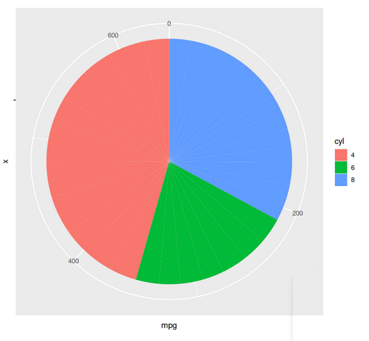
Polar Plot
This plot shows the magnitude value versus phase angle on polar coordinates.
You can polarise the plot by using the coord_polar() function.
mtcars %>%
dplyr::group_by(cyl) %>%
dplyr::summarize(mpg = median(mpg)) %>%
ggplot(aes(x = cyl, y = mpg)) + geom_col(aes(fill =cyl), color = NA)
       + labs(x = "", y = "Median mpg") + coord_polar()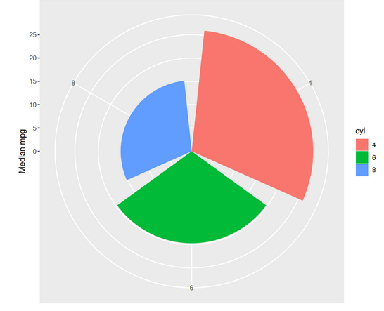
Bump Chart
A bump chart is a type of chart that displays rankings of distinct groups over time rather than absolute numbers. This is to emphasize the order of the groups rather than the amount of change.
ggplot(mtcars, aes(x = hp, y = mpg, group = cyl))
       + geom_line(aes(color = cyl), size = 2) + geom_point(aes(color = cyl), size = 4)
       + scale_y_reverse(breaks = 1:nrow(mtcars))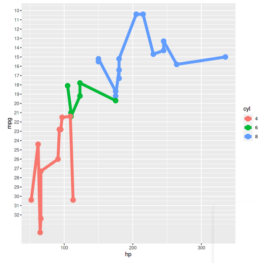
Pairplot with ggpairs
The GGally provides a function called ggpairs. This ggplot2 command is similar to the basic R pairs function. A data frame holding continuous and categorical variables can be passed.
library(GGally)
ggpairs(mtcars)
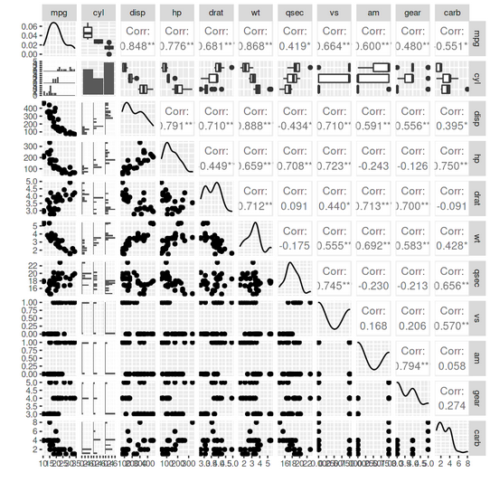
By default, the upper panel displays the correlation between the continuous variables, while the lower panel displays the scatter plots of the continuous variables. The diagonal displays the density plots of the continuous variables, and the sides display histograms and box plots for combinations of categorical and continuous variables.
The columns option is used to define the dataframe columns to be plotted. You can use either a number or a character vector containing the variable names. Use aes to create an attractive mapping. This will allow you to generate colour density plots, scatter plots, and other plots depending on the groupings.
library(GGally)
ggpairs(mtcars,columns = 1:4,aes(color = cyl, alpha = 0.5))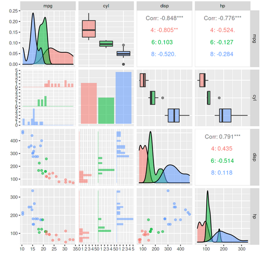
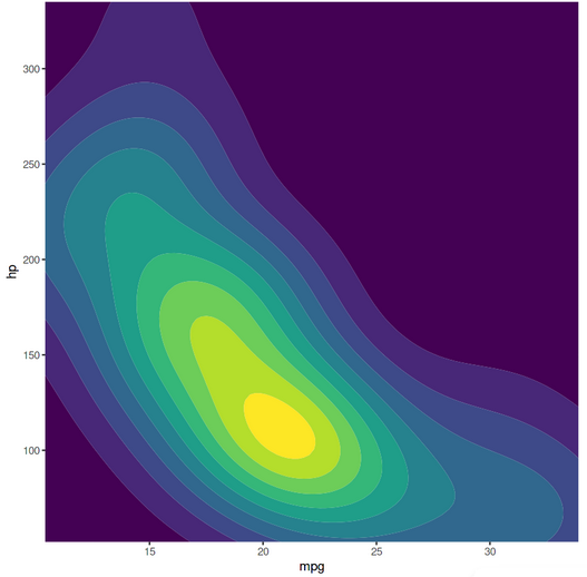
Contour Plot
ggplot2 can generate a 2D density contour plot with geom_density_2d. You only need to provide your data frame with the x and y values inside aes.
ggplot(mtcars, aes(mpg, hp)) + geom_density_2d_filled(show.legend = FALSE)
       + coord_cartesian(expand = FALSE) + labs(x = "mpg")
It’s important to note that you can make a scatter plot with contour lines. First, add the points using geom_point, & then geom_density_2d.
ggplot(mtcars, aes(x = mpg, y = hp)) + geom_point() + geom_density_2d()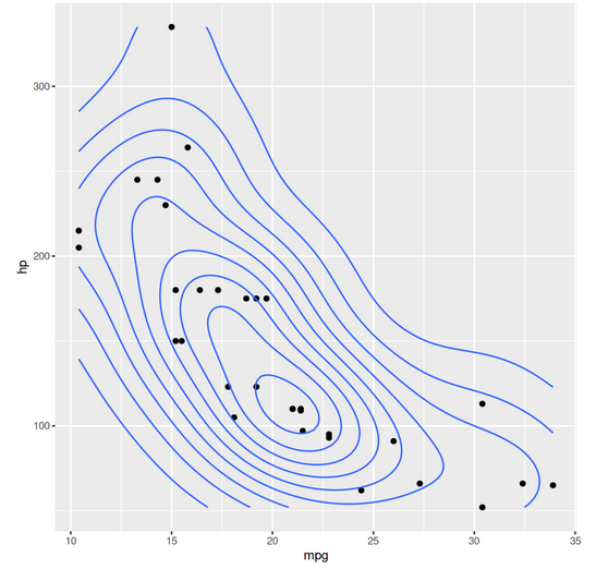
Correlogram
A correlogram, or a correlation matrix, can be created using various visualization tools in R, such as ggplot, to find the relationship between each pair of numeric variables in a dataset. It provides a high-level summary of the entire dataset, offering insights into the strength and direction of the relationships. This visual representation is particularly useful for exploratory data analysis, aiding in the identification of potential patterns or trends among variables. It is important to note that ggplot2, a powerful and versatile plotting package in R, can enhance the clarity and aesthetics of correlograms, making them valuable tools in the initial stages of data exploration.
library(ggcorrplot)
data(mtcars)
corr <- round(cor(mtcars), 1)
ggcorrplot(corr, hc.order = TRUE,
           type = "lower",
           lab = TRUE,
           lab_size = 3,
           method="circle",
           colors = c("tomato2", "white", "springgreen3"),
           title="Correlogram of mtcars",
           ggtheme=theme_bw)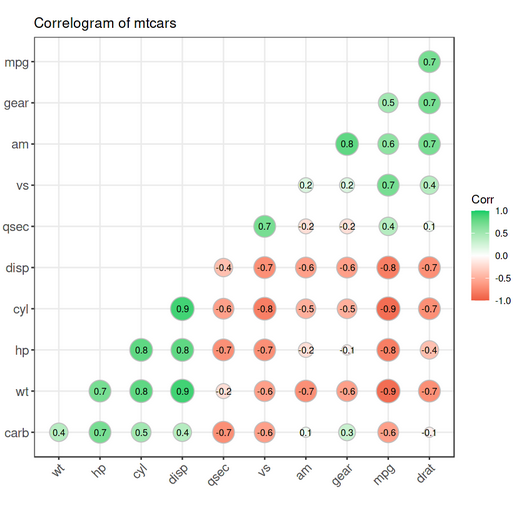
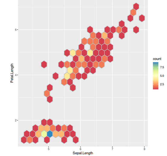
Heatmap
In ggplot2, a heat map can be built by supplying the categorical variables to the x and y parameters and the continuous variable to the fill argument of aes.
Similar to contour maps, geom_hex() may be used to display the point counts or densities that are binned to a hexagonal grid.
ggplot(iris, aes(Sepal.Length, Petal.Length)) + geom_hex(bins = 20, color = "grey")
       + scale_fill_distiller(palette = "Spectral", direction = 1)
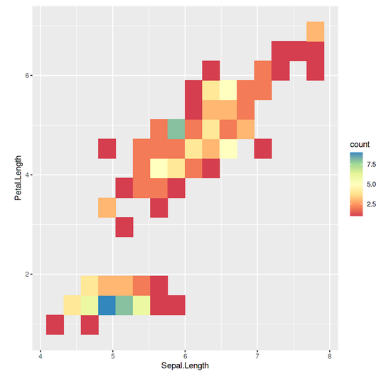
If you want a regular grid, you may use geom_bin2d(), which summarises the data into rectangular grid cells based on bins:
ggplot(iris, aes(Sepal.Length, Petal.Length)) + geom_bin2d(bins = 15)
       + scale_fill_distiller(palette = "Spectral", direction = 1)
Ridge Plot
The ggridges package’s geom_density_ridges function allows you to create a ridgeline visualization. Data Density estimation is computed and shown for each group, given a numerical variable (depth) and a categorical variable (colour).
library(ggridges)
ggplot(iris, aes(x = Sepal.Length,y= Species)) + geom_density_ridges(fill = "gray90")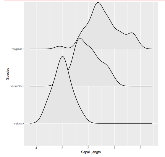
You may fill each ridgeline with a gradient by supplying stat(x) to the fill argument of aes and using geom_density_ridges_gradient and a continuous fill colour scale.
ggplot(iris, aes(x = Sepal.Length,y= Species, fill = stat(x))) + geom_density_ridges_gradient()
       + scale_fill_viridis_c(name = "Depth", option = "C")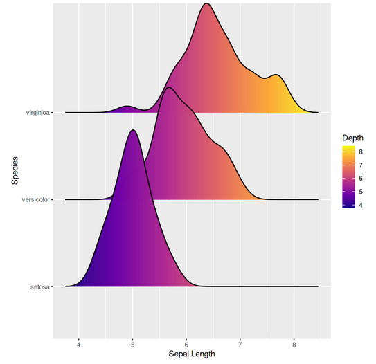
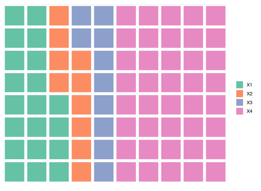
Waffle Chart
Based on ggplot2, the waffle package provides a function of the same name that can be used to make waffle charts.
Pass a vector with the count for each group to the function to generate a simple waffle plot. The plot’s number of rows can be added by using rows (defaults to 10). Choose a value based on your data.
# install.packages("waffle", repos = "https://cinc.rud.is")
library(waffle)
x <- c(X1 = 20, X2 = 10, X3 = 10,X4 = 40)
waffle(x, rows = 8)
Lime Chart
The geom_lime is a ggplot geom that draws limes in place of dots
# install.package('remotes')
remotes::install_github("coolbutuseless/geomlime")
library(geomlime)
ggplot(mtcars, aes(mpg, wt)) +geom_lime(size = 6)

Customization in ggplot2 in R
We can do a lot with ggplot2. Let’s explore it in the following sections:
Plot Titles
You can add a title, a subtitle, a caption, and a tag for your visualization when using ggplot2. There are two methods for adding titles: ggtitle and the labs function. The former is only for titles and subtitles, but the latter allows for the addition of tags and captions.
ggplot(mtcars, aes(x=as.factor(cyl), y=mpg)) + geom_boxplot()+ ggtitle("hp vs mpg")To add the title, use the labs function.
ggplot(mtcars, aes(x=as.factor(cyl), y=mpg)) + geom_boxplot() +labs(title = "hp vs mpg")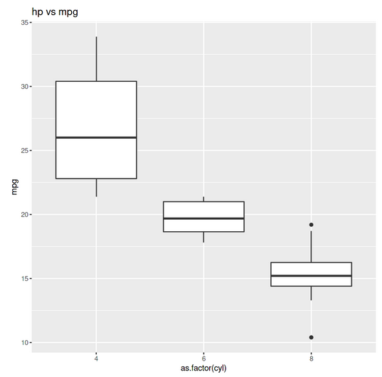
Similarly, You can add a subtitle the same way you added the title, but with the subtitle argument using the ggtitle() or labs() function:
ggplot(mtcars, aes(x=as.factor(cyl), y=mpg)) + geom_boxplot()
       + ggtitle("hp vs mpg",subtitle = "Subtitle of the plot")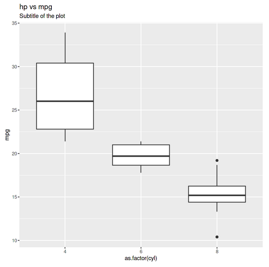
Horizontal alignment or hjust is used to control the alignment of the title (i.e., left, centre, right). Similarly, for controlling the vertical alignment, vjust can be used.
ggplot(mtcars, aes(x=as.factor(cyl), y=mpg)) + geom_boxplot()+ ggtitle("hp vs mpg")
       +theme(plot.title = element_text(hjust = 1, size = 16, face = "bold"))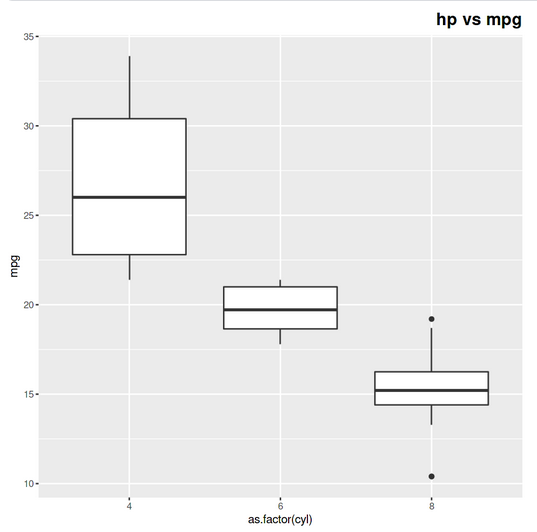
Themes
Themes in ggplot2 in R can be used to modify the background, text & legend colours, and axis text.
The ggplot2 in R package includes eight pre-installed themes. The theme() is a command for manually modifying all types of theme components, including rectangles, texts, and lines. It uses the theme named theme_gray by default, so you don’t need to define it.
The eight pre-installed themes are:
- Theme_gray (default)
- Theme_bw – This theme uses a white background, and grey coloured thin grid lines, which is the variation on theme_gray().
- Theme line draw – This theme has a white background which contains black lines only of different widths.
- Theme_light – This theme is very similar to theme_linedraw() except for the axes and light grey coloured grid lines.
- Theme_dark – This theme is the darker version of theme_light(), which has a dark background with similar line sizes. It is useful to make thin lines of different colours pop out in your graph.
- Theme_minimal – This is a simple theme with no background annotations.
- Theme_classic – This is a traditional theme with x and y-axis lines and has no gridlines.
- Theme_void – This theme is an empty theme with no content.
In ggplot2, you are not bound to the built-in themes. Other themes include the ggthemes package, the hrbrthemes package, the ggthemr package, the ggtech package, and the ggdark package.
Jeffrey Arnold’s ggthemes package includes commonly used themes. Some of them cover colour scales. Use the scales accordingly based on your data. You may alter the panel’s background colour by changing an element_rect in the panel. Select a different colour using the following command:
ggplot(mtcars, aes(x=as.factor(cyl), y=mpg)) + geom_boxplot()
       + theme(panel.background = element_rect(fill = "#72efdd"))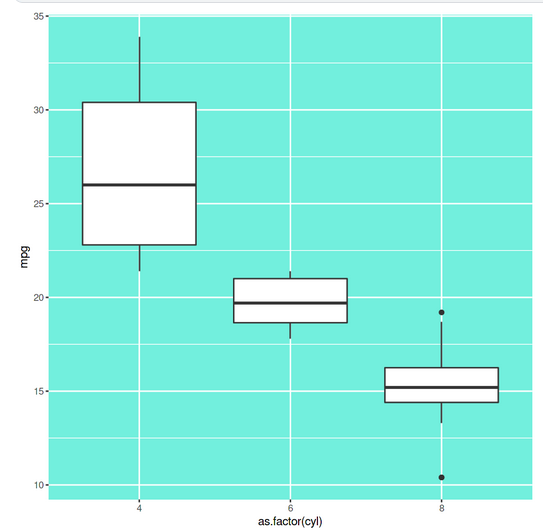
The Color and width of the border in the panel can be controlled by the ‘panel.border’ component with colour and size arguments. However, to avoid hiding the data, we must set the fill =” transparent”.
ggplot(mtcars, aes(x=as.factor(cyl), y=mpg)) + geom_boxplot()
       + theme(panel.border = element_rect(fill = "transparent", color = "#72efdd",size = 4))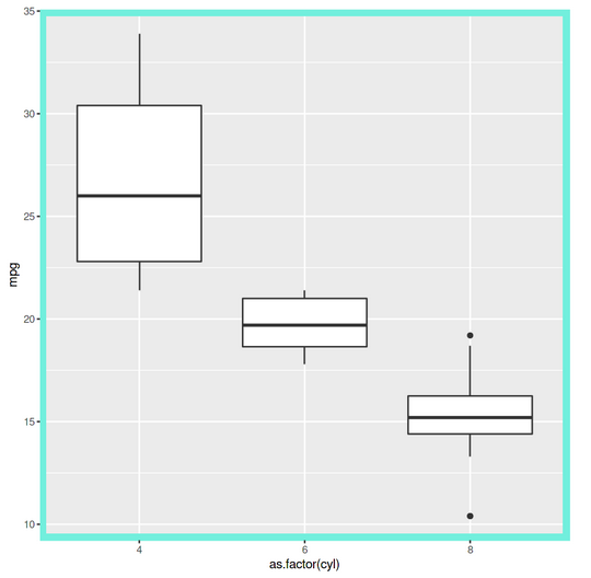
We can modify the background colour of the graph by using the theme component ‘plot.background’. Just set the Color of your choice in the fill argument of an element_rect.
ggplot(mtcars, aes(x=as.factor(cyl), y=mpg)) + geom_boxplot()
       +theme(plot.background = element_rect(fill = "#72efdd"))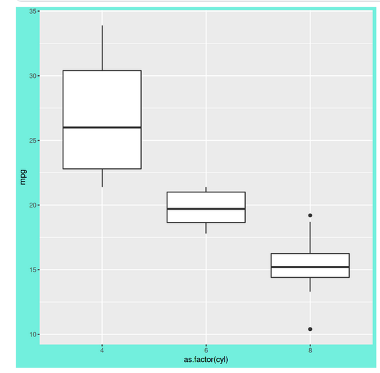
Grid Customisation
By default, ggplot2 creates a major and minor white grid. To customize the grid appearance, we need to use the theme function component ‘panel.grid’. With the element_line function’s arguments, you can change the colour, line width, and line type.
ggplot(mtcars, aes(x=as.factor(cyl), y=mpg)) + geom_boxplot()
       + theme(panel.grid = element_line(color = "#3a0ca3",size = 1,linetype = 3))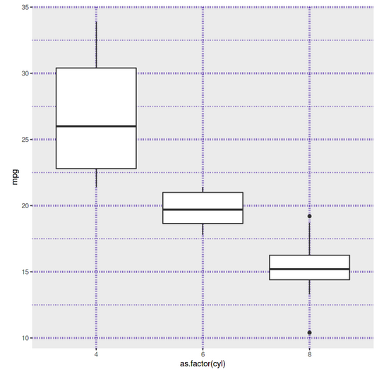
Using element_blank instead of element_line, we can remove the grid lines.
ggplot(mtcars, aes(x=as.factor(cyl), y=mpg)) + geom_boxplot()+ theme(panel.grid = element_blank())Margins
Using the margin function setting in the theme function component ‘plot.margin’, we can modify the plot margins. The labels t,r,b,l inside the margin() object refer to top, right, bottom, left, respectively. The four margins are margin(t, r, b, l).
ggplot(mtcars, aes(x=as.factor(cyl), y=mpg)) + geom_boxplot()
       + theme(plot.background = element_rect(color = 1,size = 1),
         plot.margin = margin(t = 20,r = 50,b = 40,l = 30))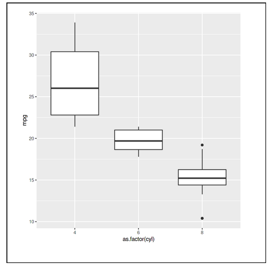
Legends
Passing a categorical (or numerical) variable to colour, fill, shape, or alpha inside aes, we can add a legend to our graph. The output will change depending on the parameter you choose to pass the data.
You can remove the legend with the following command:
theme(legend.position = "none")To place the legend at another location than the default placement on the right, you have to use the argument ‘legend.position’ in the theme. The locations available are “top,” “right” (the default), “bottom,” and “left.”
Creating a panel of different plots
Plots can be joined in a variety of ways. The patchwork package by Thomas Lin Pedersen is the simplest approach:
p1 <- ggplot(mtcars, aes(x = hp, y = mpg,color = gear)) + geom_line(color = "#3a0ca3")+geom_point()
p2 <- ggplot(mtcars, aes(x = carb, y = mpg,color = gear)) + geom_line(color = "#c9184a") +geom_point()
library(patchwork)
p1 + p2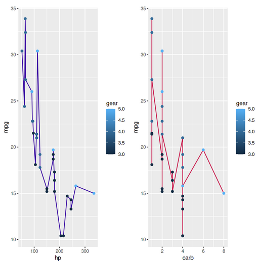
You can create subplots using gridExtra. You have to install the package, if not installed, to do the layout:
library(gridExtra)first <- ggplot(mtcars, aes(x=qsec, fill=cyl)) + geom_histogram(binwidth = 0.1)
second <- ggplot(mtcars, aes(x=wt, fill=cyl)) + geom_histogram(binwidth = 0.1)
third <- ggplot(mtcars, aes(x=gear, fill=cyl)) + geom_histogram(binwidth = 0.1)
fourth <- ggplot(mtcars, aes(x=carb, fill=cyl)) + geom_histogram(binwidth = 0.1)
grid.arrange(first,second,third,fourth, nrow = 2)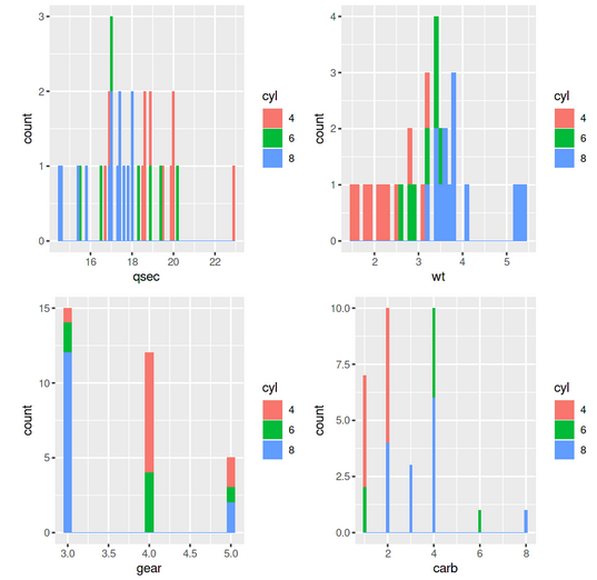
Faceting
Faceting is used to plot graphs for different categories of a specific variable. Let us try to understand it with an example:
unique(mtcars$carb)
We can see that “carb” is divided into six groups. Faceting generates six plots between mpg and hp, with the dots representing the categories.
ggplot(mtcars, aes(hp,mpg)) + geom_point()+facet_wrap(~carb)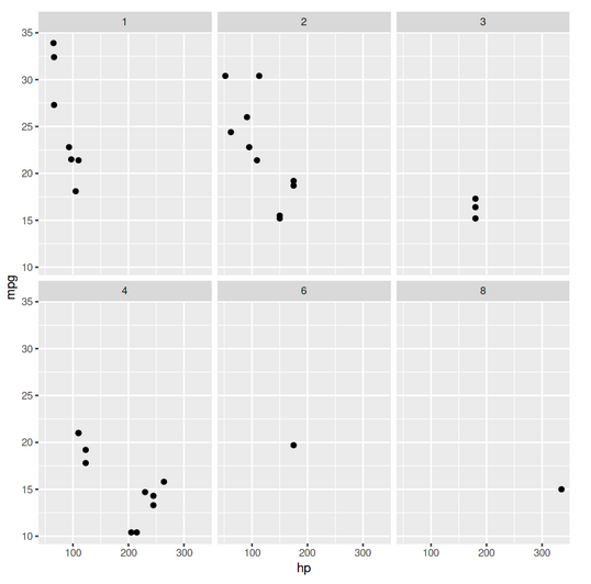
The facet wrap function is used for faceting, where the variables to be classified are defined after the tilde(~) symbol.
Faceting can be done by using the facet_grid function, which can be used to face in two dimensions.
ggplot(mtcars, aes(hp,mpg)) + geom_point()+ facet_grid(. ~ cyl)+ facet_grid(cyl ~ .)
       + facet_grid(gear ~ cyl,labeller = "label_both")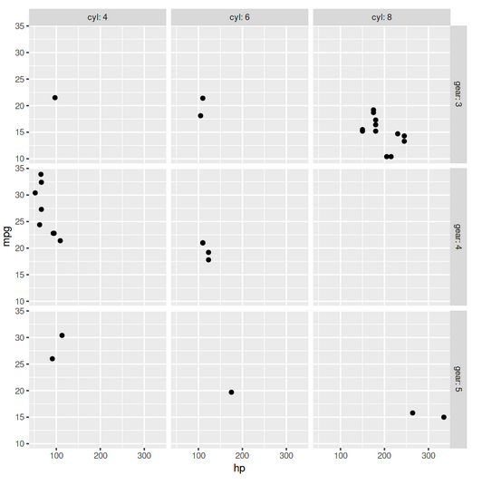
Conclusion
Although there are multiple libraries in R like ggvis and htmlwidgets, which allow interactive charts, the ggplot2 in R package is still one of the most commonly used packages in R for static data visualization. The plotly package can be used to make the ggplot2 chart interactive.
In this guide, we saw several different types of plots using the ggplot2 library and how to customize these plots easily in R. The code for this guide is available on my GitHub repository. Feel free to try these visualizations on another dataset.
Hope you liked my article on ggplot2 in R. Share with me in the comments below.
Read the latest articles on our blog.
Frequently Asked Questions
A. ggplot is a popular data visualization package in R programming. It stands for “Grammar of Graphics plot” and is based on the grammar of graphics concept, which provides a consistent and structured way to create visualizations. ggplot is used for creating a wide range of high-quality and customizable statistical graphs, such as scatter plots, bar charts, line plots, histograms, and more, to effectively explore and present data.
A. ggplot2, developed by Hadley Wickham in R, is a powerful plotting library inspired by Leland Wilkinson’s book “The Grammar of Graphics.” The name “gg” represents “Grammar of Graphics.”
The media shown in this article is not owned by Analytics Vidhya and are used at the Author’s discretion.


This is an article I use over and over again. Thank you for sharing your insigth.
It is indeed a very informative article. Thank you. I have only one issue. When I try to create the "Subplots with gridExtra", the histograms are black and white and I get the following warning message: "The following aesthetics were dropped during statistical transformation: fill. ℹ This can happen when ggplot fails to infer the correct grouping structure in the data. ℹ Did you forget to specify a `group` aesthetic or to convert a numerical variable into a factor?" Any suggestion?