Building Naive Bayes Classifier from Scratch to Perform Sentiment Analysis
This article was published as a part of the Data Science Blogathon.
Introduction
In my last article (Sentiment Analysis with LSTM), we discGranger Causality in Time Series Explained with Chickenussed what sentiment analysis is and how to perform it using LSTM. LSTM is a deep-learning-based classifier, and it takes a considerable amount of time to train it. In this article, we will explore a faster machine learning classifier – the Naive Bayes classifier, which uses the Bayes’ theorem to classify new test examples into one of the previously defined classes. We will learn how to build the Naive Bayes classifier from scratch rather than using libraries, and use it to classify movie reviews of the same IMDB dataset we had used in the last article. Let us dive right in!
Source : ImageLink
What is a Naive Bayes Classifier?
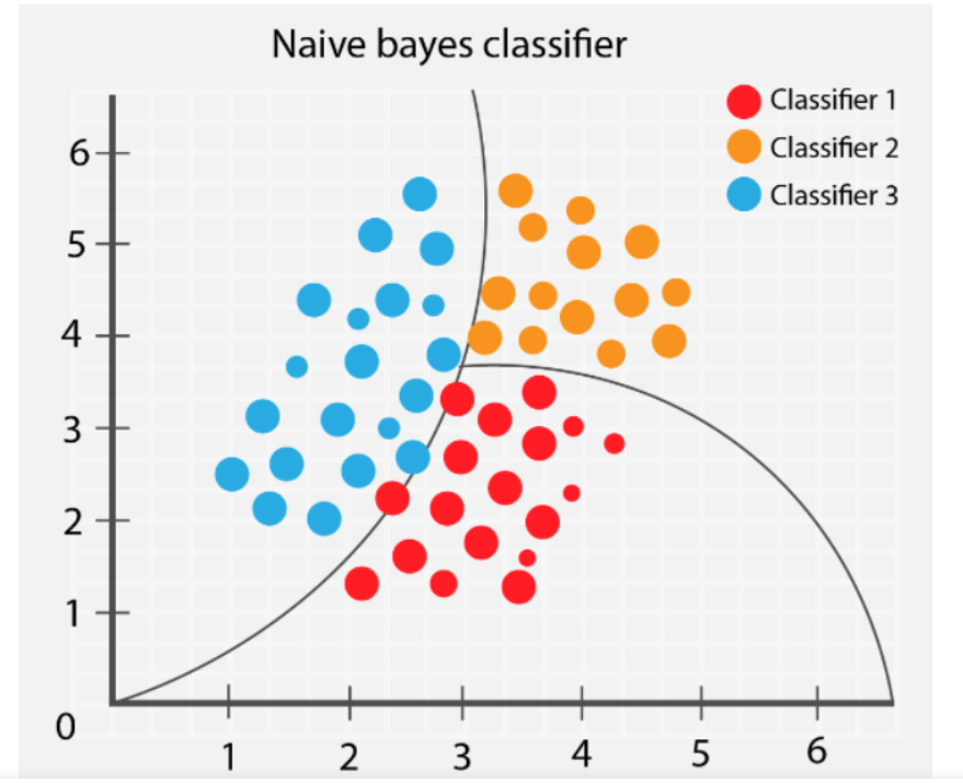
The Naive Bayes algorithm is a supervised machine learning algorithm based on the Bayes’ theorem. It is a probabilistic classifier that is often used in NLP tasks like sentiment analysis (identifying a text corpus’ emotional or sentimental tone or opinion).
The Bayes’ theorem is used to determine the probability of a hypothesis when prior knowledge is available. It depends on conditional probabilities. The formula is given below :
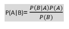
where P(A|B) is posterior probability i.e. the probability of a hypothesis A given the event B occurs. P(B|A) is likelihood probability i.e. the probability of the evidence given that hypothesis A is true. P(A) is prior probability i.e. the probability of the hypothesis before observing the evidence and P(B) is marginal probability i.e. the probability of the evidence. When the Bayes’ theorem is applied to classify text documents, the class c of a particular document d is given by :
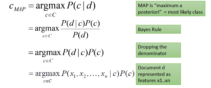
Let the feature conditional probabilities P(x_i | c) be independent of each other (conditional independence assumption). So,
P(x_1, x_2, …, x_n | c) = P(x_1 | c) X P(x_2 | c) X … X P(x_n | c)
Now, if we consider words as the features of the document, the individual feature conditional probabilities can be calculated using the following formula :
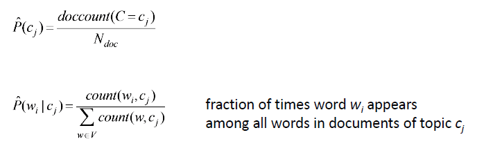
But what if a given word w_i does not occur in any training document of class c_j, but it appears in a text document? P(w_i | c_j) will become 0, which means the probability of the test document belonging to class c_j will become 0. To avoid this, Laplace smoothing is introduced and the conditional feature probabilities are actually calculated in the following way :
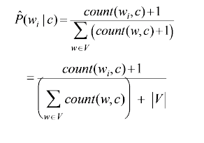
where |V| is the number of unique words in the text corpus. This way we can easily deal with unseen test words.
Now that we know how Naive Bayes classifiers work, let us start building our own NB classifier from scratch.
Loading the Dataset
We will perform sentiment analysis on the IMDB dataset, which has 25k positive and 25k negative movie reviews. We need to build an NB classifier that classifies an unseen movie review as positive or negative. The dataset can be downloaded from here. Let us start by importing necessary packages for text manipulation and loading the dataset into a pandas dataframe :
import re

import pandas as pd

import numpy as np

from sklearn.preprocessing import LabelEncoder

from sklearn.model_selection import train_test_split

from sklearn.metrics import classification_report

from sklearn.metrics import accuracy_score

import math

import nltk

from sklearn.feature_extraction.text import CountVectorizer

from collections import defaultdict

data = pd.read_csv('IMDB Dataset.csv')

data
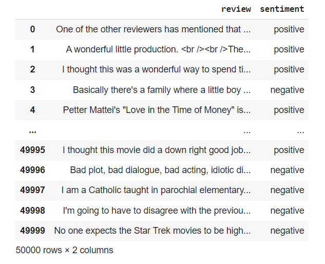
Source: Screenshot from my Jupyter Notebook
Data Preprocessing
We remove HTML tags, URLs and non-alphanumeric characters from the dataset using regex functions. Stopwords (commonly used words like ‘and’, ‘the’, ‘at’ that do not hold any special meaning in a sentence) are also removed from the corpus using the nltk stopwords list :
def remove_tags(string):
    removelist = ""
    result = re.sub('','',string)          #remove HTML tags
    result = re.sub('https://.*','',result)   #remove URLs
    result = re.sub(r'[^w'+removelist+']', ' ',result)    #remove non-alphanumeric characters
    result = result.lower()
    return result
data['review']=data['review'].apply(lambda cw : remove_tags(cw))
nltk.download('stopwords')
from nltk.corpus import stopwords
stop_words = set(stopwords.words('english'))
data['review'] = data['review'].apply(lambda x: ' '.join([word for word in x.split() if word not in (stop_words)]))
Finally, we perform lemmatization on the text. Lemmatization is used to find the root form of words or lemmas in NLP. For example, the lemma of the words reading, reads, read is read. This helps save unnecessary computational overhead in trying to decipher entire words since the meanings of most words are well-expressed by their separate lemmas. We perform lemmatization using the WordNetLemmatizer() from nltk. The text is first broken into individual tokens/ words using the WhitespaceTokenizer() from nltk. We write a function lemmatize_text to perform lemmatization on the individual words.
w_tokenizer = nltk.tokenize.WhitespaceTokenizer()
lemmatizer = nltk.stem.WordNetLemmatizer()
def lemmatize_text(text):
    st = ""
    for w in w_tokenizer.tokenize(text):
        st = st + lemmatizer.lemmatize(w) + " "
    return st
data['review'] = data.review.apply(lemmatize_text)
The dataset looks like this after preprocessing :
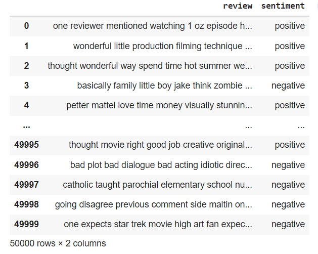
Source: Screenshot from my Jupyter Notebook
Encoding Labels and Making Train-Test Splits
LabelEncoder() from sklearn.preprocessing is used to convert the labels (‘positive’, ‘negative’) into 1’s and 0’s respectively.
reviews = data['review'].values
labels = data['sentiment'].values
encoder = LabelEncoder()
encoded_labels = encoder.fit_transform(labels)
The dataset is then split into 80% train and 20% test parts using train_test_split from sklearn.model_selection.
train_sentences, test_sentences, train_labels, test_labels = train_test_split(reviews, encoded_labels, stratify = encoded_labels)
Building the Naive Bayes Classifier
Many variants of the Naive Bayes classifier are available in the sklearn library. However, we are going to be building our own classifier from scratch using the formulas described earlier. We start by using the CountVectorizer from sklearn.feature_extraction.text to get the frequency of each word appearing in the training set. We store them in a dictionary called ‘word_counts’. All the unique words in the corpus are stored in ‘vocab’.
vec = CountVectorizer(max_features = 3000)
X = vec.fit_transform(train_sentences)
vocab = vec.get_feature_names()
X = X.toarray()
word_counts = {}
for l in range(2):
    word_counts[l] = defaultdict(lambda: 0)
for i in range(X.shape[0]):
    l = train_labels[i]
    for j in range(len(vocab)):
        word_counts[l][vocab[j]] += X[i][j]
As we mentioned earlier, we need to perform Laplace smoothing to handle words in the test set which are absent in the training set. We define a function ‘laplace_smoothing’ which takes the vocabulary and the raw ‘word_counts’ dictionary and returns the smoothened conditional probabilities.
def laplace_smoothing(n_label_items, vocab, word_counts, word, text_label):
    a = word_counts[text_label][word] + 1
    b = n_label_items[text_label] + len(vocab)
    return math.log(a/b)
We define the ‘fit’ and ‘predict’ functions for our classifier.
def group_by_label(x, y, labels):
    data = {}
    for l in labels:
        data[l] = x[np.where(y == l)]
    return data
def fit(x, y, labels):
    n_label_items = {}
    log_label_priors = {}
    n = len(x)
    grouped_data = group_by_label(x, y, labels)
    for l, data in grouped_data.items():
        n_label_items[l] = len(data)
        log_label_priors[l] = math.log(n_label_items[l] / n)
     return n_label_items, log_label_priors
The ‘fit’ function takes x (reviews) and y (labels – ‘positive’, ‘negative’) values to be fitted on and returns the number of reviews with each label and the apriori conditional probabilities. Finally, the ‘predict’ function is written which returns predictions on unseen test reviews.
def predict(n_label_items, vocab, word_counts, log_label_priors, labels, x):
    result = []
    for text in x:
        label_scores = {l: log_label_priors[l] for l in labels}
        words = set(w_tokenizer.tokenize(text))
        for word in words:
            if word not in vocab: continue
            for l in labels:
                log_w_given_l = laplace_smoothing(n_label_items, vocab, word_counts, word, l)
                label_scores[l] += log_w_given_l
        result.append(max(label_scores, key=label_scores.get))
    return result
Fitting the Model on Training Set and Evaluating Accuracies on the Test Set
The classifier is now fitted on the train_sentences and is used to predict labels for the test_sentences. The accuracy of the prediction on the test set comes out to be 85.16%, which is pretty good. We calculate accuracy using ‘accuracy_score’ from sklearn.metrics.
labels = [0,1]
n_label_items, log_label_priors = fit(train_sentences,train_labels,labels)
pred = predict(n_label_items, vocab, word_counts, log_label_priors, labels, test_sentences)
print("Accuracy of prediction on test set : ", accuracy_score(test_labels,pred))
Frequently Asked Questions
A. In sentiment analysis, Naive Bayes is utilized to classify text sentiment. The approach assumes features (words) are independent given the sentiment. It calculates the probability of a text belonging to each sentiment class based on word frequencies. Then, it assigns the class with the highest probability. Despite its simplicity, Naive Bayes often performs well in sentiment analysis by quickly capturing word patterns associated with different sentiments.
A. Several algorithms are employed for sentiment analysis, including:
1. Naive Bayes: Simple and efficient, assumes word independence.
2. Support Vector Machines (SVM): Separates sentiment classes using a hyperplane.
3. Logistic Regression: Estimates the probability of a sentiment class.
4. Deep Learning (e.g., LSTM, CNN): Processes text data using neural networks, capturing complex patterns.
5. Random Forest: Uses an ensemble of decision trees for sentiment classification.
6. Gradient Boosting: Boosts the predictive power of weak models, enhancing sentiment analysis accuracy.
7. Word Embeddings (e.g., Word2Vec, GloVe): Converts words to vectors, preserving semantic relationships for sentiment understanding.
Conclusion
In this article, we learnt what is a Naive Bayes classifier and how to build it from scratch. You can now use the classifier to predict the label for unseen movie reviews not present in the dataset. Note that there are readymade Naive Bayes models available in the scikit-learn library which we can use in our work instead of building models from scratch. There are 5 types of Naive Bayes classifiers available in scikit-learn – namely Bernoulli Naive Bayes, Categorical NB, Complement NB, Gaussian NB, and Multinomial NB. You can learn more about them here.
The key takeaways from this article are :
- A Naive Bayes classifier is a probabilistic ML classifier based on the Bayes theorem.
- We can build our own NB classifier from scratch and use it for text classification like sentiment analysis or spam filtering.
- Laplace smoothing needs to be performed while calculating feature conditional probabilities so that we are able to handle unseen test words not present in the training corpus.
Thank you for reading.
You can read here about how to use CNNs in NLP!
Feel free to connect with me over email: [email protected]
The media shown in this article is not owned by Analytics Vidhya and are used at the Author’s discretion.


