Music Genre Classification Project Using Machine Learning Techniques

This article was published as a part of the Data Science Blogathon.

Hello, and welcome to a wonderful article on audio classification. Audio classification is an Application of machine learning where different sound is categorized in certain categories. In our previous blog, we have studied Audio classification using ANN and build a model from scratch. Almost all data science enthusiasts want attractive and eye-catching data science projects on their resume and Audio processing is one such topic. In this project, we will build a complete music Genre classification project from scratch using a machine learning algorithm known as the K-Nearest Neighbors classification algorithm.

Table of Contents

1. Introduction to Music Genre Classification
2. Project Overview
3. System Prerequisites
   • Overview of Dataset
   • Libraries Installation
4. Implement music genre classification from scratch
5. Test New Audio Files
6. Conclusion

Introduction to Music Genre Classification

Audio processing is one of the most complex tasks in data science as compared to image processing and other classification techniques. One such application is music genre classification which aims to classify the audio files in certain categories of sound to which they belong. The application is very important and requires automation to reduce the manual error and time because if we have to classify the music manually then one has to listen out each file for the complete duration. So To automate the process we use Machine learning and deep learning algorithms and this is what we will implement in this article.

Project Overview and Approach

In short, we can define our project problem statement as like given multiple audio files, and the task is to categorize each audio file in a certain category like audio belongs to Disco, hip-hop, etc. The music genre classification can be built using different approaches in which the top 4 approaches that are mostly used are listed below.

1. Multiclass support vector machine
2. K-Nearest Neighbors
3. K-means clustering algorithm
4. Convolutional neural network

We will use K-Nearest Neighbors algorithm because various researches prove it is one of the best algorithms to give good performance and till time along with optimized models organizations uses this algorithm in recommendation systems as support.

K-Nearest Neighbour ~ KNN is a machine learning algorithm used for regression, and classification. It is also known as the lazy learner algorithm. It simply uses a distance-based method o find the K number of similar neighbours to new data and the class in which the majority of neighbours lies, it results in that class as an output. Now let us get our system ready for project implementation.

Dataset Overview

The dataset we will use is named the GTZAN genre collection dataset which is a very popular audio collection dataset. It contains approximately 1000 audio files that belong to 10 different classes. Each audio file is in .wav format (extension). The classes to which audio files belong are Blues, Hip-hop, classical, pop, Disco, Country, Metal, Jazz, Reggae, and Rock. You can easily find the dataset over Kaggle and can download it from here. If you do not have much memory space then you can create a Kaggle notebook and practice it there.

Libraries Installation

Before we move to load dataset and model building it’s important to install certain libraries. In the last blog, we have used librosa to extract features. Now we will use the python speech feature library to extract features and to have a different taste. as well as to load the dataset in the WAV format we will use the scipy library so we need to install these two libraries.

!pip install python_speech_features
!pip install scipy

Hands-on Implementation of Music Genre Classification PProject

Step-1) Import required libraries

Head over to Jupyter notebook or newly created Kaggle notebook and first thing is to make necessary imports to play with the data.

import numpy as np
import pandas as pd
import scipy.io.wavfile as wav
from python_speech_features import mfcc
from tempfile import TemporaryFile
import os
import math
import pickle
import random
import operator

Step-2) Define a function to calculate distance between feature vectors, and to find neighbours.

We know how KNN works is by calculating distance and finding the K number of neighbours. To achieve this only for each functionality we will implement different functions. First, we will implement a function that will accept training data, current instances, and the required number of neighbours. It will find the distance of each point with every other point in training data and then we find all the nearest K neighbours and return all neighbours. to calculate the distance of two-point we will implement a function after explaining some steps to make a project workflow simple and understandable.

#define a function to get distance between feature vectors and find neighbors
def getNeighbors(trainingset, instance, k):
    distances = []
    for x in range(len(trainingset)):
        dist = distance(trainingset[x], instance, k) + distance(instance,trainingset[x],k)
        distances.append((trainingset[x][2], dist))
    distances.sort(key=operator.itemgetter(1))
    neighbors = []
    for x in range(k):
        neighbors.append(distances[x][0])
    return neighbors

Step-3) Identify the class of nearest neighbours

Now we are having a list of neighbours and we need to find out a class that has the maximum neighbours count. So we declare a dictionary that will store the class and its respective count of neighbours. After creating the frequency map we sort the map in descending order based on neighbours count and return the first class.

#function to identify the nearest neighbors
def nearestclass(neighbors):
    classVote = {}
    
    for x in range(len(neighbors)):
        response = neighbors[x]
        if response in classVote:
            classVote[response] += 1
        else:
            classVote[response] = 1
            
    sorter = sorted(classVote.items(), key=operator.itemgetter(1), reverse=True)
    return sorter[0][0]

Step-4) Model Evaluation

we also require a function that evaluates a model to check the accuracy and performance of the algorithm we build. so we will build a function that is a fairly simple accuracy calculator which says a total number of correct predictions divided by a total number of predictions.

def getAccuracy(testSet, prediction):
    correct = 0
    for x in range(len(testSet)):
        if testSet[x][-1] == prediction[x]:
            correct += 1
    return 1.0 * correct / len(testSet)

Step-5) Feature Extraction

you might be thinking like we have implemented the model and now we will extract features from data. So as we are using KNN Classifier and we have only implemented the algorithm from scratch to make you understand how the project runs and till now I hope you have a 70 percent of idea how the project will work. So now we will load the data from all the 10 folders of respective categories and extract features from each audio file and save the extracted features in binary form in DAT extension format.

Mel Frequency Cepstral Coefficients

Feature extraction is a process to extract important features from data. It includes identifying linguistic data and avoiding any kind of noise. Audio features are classified into 3 categories high-level, mid-level, and low-level audio features.

• High-level features are related to music lyrics like chords, rhythm, melody, etc.
• Mid-level features include beat level attributes, pitch-like fluctuation patterns, and MFCCs.
• Low-level features include energy, a zero-crossing rate which are statistical measures that get extracted from audio during feature extraction.

So to generate these features we use a certain set of steps and are combined under a single name as MFCC that helps extract mid-level and low-level audio features. below are the steps discussed for the working of MFCCs in feature extraction.

1. Audio files are of a certain length(duration) in seconds or as long as in minutes. And the pitch or frequency is continuously changing so to understand this we first divide the audio file into small-small frames which are near about 20 to 40 ms long.
2. After dividing into frames we try to identify and extract different frequencies from each frame. When we divide in such a small frame so assume that one frame divides down in a single frequency.
3. separate linguistic frequencies from the noise
4. To discard any type of noise, take discrete cosine transform (DCT) of the frequencies. students who are from engineering backgrounds might know cosine transform and have studied this in discrete mathematics subjects.

Now we do not have to implement all these steps separately, MFCC brings all these for us which we have already imported from the python speech feature library. we will iterate through each category folder, read the audio file, extract the MFCC feature, and dump it in a binary file using the pickle module. I suggest always using try-catch while loading huge datasets to understand, and control if any exception occurs.

directory = '../input/gtzan-dataset-music-genre-classification/Data/genres_original'
f = open("mydataset.dat", "wb")
i = 0
for folder in os.listdir(directory):
    #print(folder)
    i += 1
    if i == 11:
        break
    for file in os.listdir(directory+"/"+folder):
        #print(file)
        try:
            (rate, sig) = wav.read(directory+"/"+folder+"/"+file)
            mfcc_feat = mfcc(sig, rate, winlen = 0.020, appendEnergy=False)
            covariance = np.cov(np.matrix.transpose(mfcc_feat))
            mean_matrix = mfcc_feat.mean(0)
            feature = (mean_matrix, covariance, i)
            pickle.dump(feature, f)
        except Exception as e:
            print("Got an exception: ", e, 'in folder: ', folder, ' filename: ', file)
f.close()

Step-6) Train-test split the dataset

Now we have extracted features from the audio file which is dumped in binary format as a filename of my dataset. Now we will implement a function that accepts a filename and copies all the data in form of a dataframe. After that based on a certain threshold, we will randomly split the data into train and test sets because we want a mix of different genres in both sets. There are different approaches to do train test split. here I am using a random module and running a loop till the length of a dataset and generate a random fractional number between 0-1 and if it is less than 66 then a particular row is appended in the train test else in the test set.

dataset = []

def loadDataset(filename, split, trset, teset):
    with open('my.dat','rb') as f:
        while True:
            try:
                dataset.append(pickle.load(f))
            except EOFError:
                f.close()
                break
    for x in range(len(dataset)):
        if random.random() < split:
            trset.append(dataset[x])
        else:
            teset.append(dataset[x])

trainingSet = []
testSet = []
loadDataset('my.dat', 0.68, trainingSet, testSet)

Step-7) Calculate the distance between two instance

This function we have to implement at the top to calculate the distance between two points but to explain to you the complete workflow of the project, and algorithm I am explaining the supporting function after the main steps. But you need to add the function on top. So, the function accepts two data points(X, and y coordinates) to calculate the actual distance between them. we use the numpy linear algebra package which provides a low-level implementation of standard linear algebra. So we first find the dot product between the X-X and Y-Y coordinate of both points to know the actual distance after that we extract the determinant of the resultant array of both points and get the distance.

def distance(instance1, instance2, k):
    distance = 0
    mm1 = instance1[0]
    cm1 = instance1[1]
    mm2 = instance2[0]
    cm2 = instance2[1]
    distance = np.trace(np.dot(np.linalg.inv(cm2), cm1))
    distance += (np.dot(np.dot((mm2-mm1).transpose(), np.linalg.inv(cm2)), mm2-mm1))
    distance += np.log(np.linalg.det(cm2)) - np.log(np.linalg.det(cm1))
    distance -= k
    return distance

Step-8)  Training the Model and making predictions

The step has come you all were waiting to feed the data to KNN algorithms and make all predictions and receive accuracy on the test dataset. This step code seems to be large but it is very small because we are following a functional programming approach in a stepwise manner so we only need to call the functions. The first is to get neighbors, extract class and check the accuracy of the model.

# Make the prediction using KNN(K nearest Neighbors)
length = len(testSet)
predictions = []
for x in range(length):
    predictions.append(nearestclass(getNeighbors(trainingSet, testSet[x], 5)))

accuracy1 = getAccuracy(testSet, predictions)
print(accuracy1)

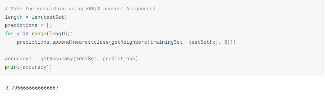
Image Source – SS By Author

Step-9) Test the Classifier with the new Audio File

Now we have implemented and trained the model and it’s time to check for the new data to check how much our model is compliant in predicting the new audio file. So we have all the labels (classes) in numeric form, and we need to check the class name so first, we will implement a dictionary where the key is numeric label and value is the category name.

from collections import defaultdict
results = defaultdict(int)

directory = "../input/gtzan-dataset-music-genre-classification/Data/genres_original"

i = 1
for folder in os.listdir(directory):
    results[i] = folder
    i += 1

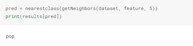
Now we can predict a new audio file and receive a label for it and print the name of the category using the result dictionary.

Conclusion

Hurray! congratulations to you if you have implemented the project till the end. We have started the project with the initial setup and used MFCC to extract features from audio files. After that, we have built a KNN classifier from scratch that finds K number of nearest neighbour based on features and maximum neighbour belonging to particular class gives as an output. We got approximately 70 per cent accuracy on the model. Let us summarize the major key takeaways we have learned while implementing this project and what is the future scope of the project.

1. The main thing to identify and divide the audio into different features is amplitude and frequency that changes within a short span of time.
2. We can visualize the audio frequency wave of amplitude and frequency with respect to time in form of a wave plot that can be easily plotted using librosa.
3. MFCCs total provides 39 features related to frequency and amplitude. In that 12 parameters are related to the amplitude of frequencies. It means it provides us with enough frequency channels to analyze audio and this is the reason MFCCs are used everywhere for feature extraction in audios.
4. The key working of MFCC is to remove vocal excitation (pitch information) by dividing audio into frames, make extracted features independent, adjust the loudness, and frequency of sound according to humans, and capture the context.

👉 The complete Notebook implementation is available here.

👉 I hope that it was easy to cope-up with each step and easily understandable. If you have any queries then feel free to post them in the comment section below or can connect with me.

👉 Connect with me on Linkedin.

👉 Check out my other articles on Analytics Vidhya and crazy-techie

Thanks for giving your time!

The media shown in this article is not owned by Analytics Vidhya and are used at the Author’s discretion. 

Raghav Agrawal 06 Apr 2022

I am a final year undergraduate who loves to learn and write about technology. I am a passionate learner, and a data science enthusiast. I am learning and working in data science field from past 2 years, and aspire to grow as Big data architect.