An End-to-End Guide on Time Series Forecasting Using FbProphet
This article was published as a part of the Data Science Blogathon.

Introduction to Time Series Forecasting
This article will implement time series forecasting using the Prophet library in python. The prophet is a package that facilitates the simple implementation of time series analysis.
Implementing time series forecasting can be complicated depending on the model we use. Many approaches are available for time series forecasting, for example, ARIMA ( Auto-Regressive Integrated Moving Average), Auto-Regressive Model, Exponential Smoothing, and deep learning-based models like LSTM ( long short term memory).
Time series data are those data that change over time, and predicting the future values is called time series forecasting.
For example- Forecasting stock price, user traffic on a website over time, etc.
There could be multiple ways to perform time-series forecasting, ie.ARIMA ( Auto-Regressive Integrated Moving Average), Auto-Regressive Model, Exponential Smoothing, and deep learning-based model like LSTM ( long short term memory).
There are some key concepts associated with time series forecasting-
SeasonalityIn simple terms, Seasonality means repetition over time. For example, while predicting electricity bills will be higher every year in the summer season.TrendIt tells increasing or decreasing trends over time in the data.
Facebook Prophet Library
Using Fbprophet or other time-series libraries like darts solves this problem by automating minor tweaking on their side.
Fb Prophet library was launched by Facebook now meta, and it was built for time series analysis.
Prophet library can automatically manage parameters related to seasonality and data stationarity.
This article will use the Fbprophet library for time series forecasting. While implementing the Classical time series model needs tweaking, forecasting is a bit complex.
I am implementing time series forecasting in Python.
Time series forecasting can be of two types:
- Multivariate time series means a time series dataset where the target value is determined by more than one column. For example, predicting house electricity bills depends on the season and temperature conditions.
- Univariate time series means a time series data where only a single column determines the output values, which is the date.
Loading the Dataset
In this tutorial, we will use the AV April Jobathon dataset. The dataset can be downloaded using this link.
import pandas
from matplotlib import pyplot
training_data = pandas.read_csv('../input/jobathon-april-2022/train_E1GspfA.csv')
training_data.shape

The dataset contains
- date ( parsed date)
- hour ( specific hours 1–23)
- demand ( number of rented cars)
Our job is to forecast the demand for the future time.
print(f"starting date : {str(training_data['date'].dt.date.min())}")
print(f"end date : {str(training_data['date'].dt.date.max())}")

Feature Engineering
Instead of having a separate column for the hour, we combine the hour with the date converting it into the date-time stamp.
def dataPreprocessing(dataFrame):
    dataFrame['date'] = pd.to_datetime(dataFrame['date']) + dataFrame['hour'].astype('timedelta64[h]')
    dataFrame.drop(columns=['hour'], axis=1, inplace=True)
    return dataFrame
calling the data preprocessing function
training_data = dataPreprocessing(training_data)
training_data.head()

Exploratory Data Analysis
Performing Exploratory Data Analysis helps get insight into the data, i.e. Seasonality, trend, etc.
Visualising the time series gives us the idea of seasonality, trend, etc.
fig = xp.line(training_data, x='date', y='demand')
fig.update_xaxes(rangeslider_visible=True)
fig.show()
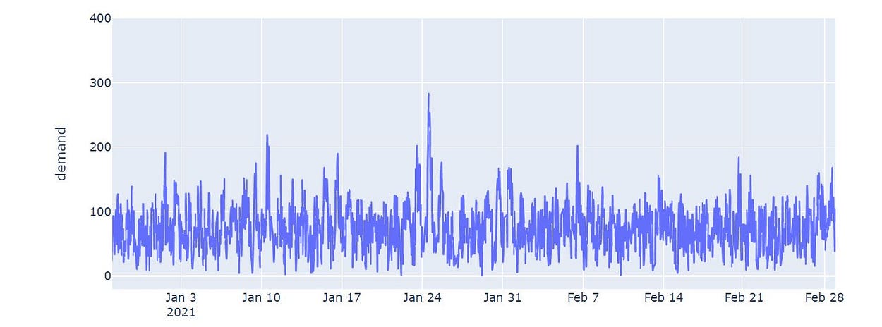
Note that the demand has some seasonality. It has a continuous repeating pattern.
Splitting the Data
Splitting the data into the training and validation part for training.
Prophet library takes date-time as a columnds and the output column as a column. y.
from sklearn.model_selection import train_test_split
import matplotlib.pyplot
training_data.rename(columns={'date': 'ds', 'demand': 'y'}, inplace=True)
train_data = training_data.sample(frac=0.8, random_state=10)
validation_data = training_data.drop(train_data.index)

print(f'training data size : {train_data.shape}')
print(f'validation data size : {validation_data.shape}')

train_data = train_data.reset_index()
validation_data = validation_data.reset_index()

Model Training
We build a prophet model and train on training data in this step.
Installing Prophet
Prophet library can be easily installed using a python package manager.
!pip install fbprophet
from sklearn.metrics import mean_absolute_error
from fbprophet import Prophet
Once installed, we can fit the Prophet model with our training data having ds and y column.
model = Prophet()
model.fit(train_data)
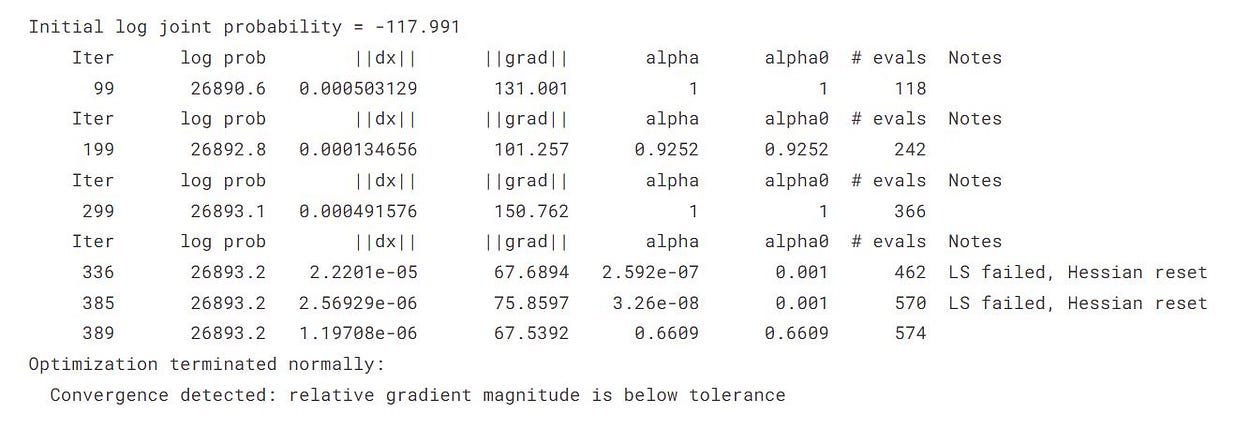
After training, the Prophet returns a window containing all the parameters and changepoints.
Model Evaluation
We will use the validation data to evaluate our model. We use mean absolute error to measure how our model is trained.
prediction = model.predict(pd.DataFrame({'ds':validation_data['ds']}))
y_actual = validation_data['y']
y_predicted = prediction['yhat']
y_predicted = y_predicted.astype(int)
mean_absolute_error(y_actual, y_predicted)

It gave 29.68. it means the average error in our actual value and the predicted value is 29.68.
We can plot the forecasted results and compare them with the actual values.
We are using Plotly interactive plots for visualisation.
from plotly.subplots import make_subplots
fig = make_subplots(specs=[[{"secondary_y": True}]])
fig.add_trace(
    go.Scatter(x=validation_data['ds'], y=y_actual, name="actual targets"),
    secondary_y=False,)
fig.add_trace(
    go.Scatter(x=validation_data['ds'], y=y_predicted, name="predicted targets"),
    secondary_y=True,)
fig.update_layout(
    title_text="Actual vs Predicted Targets")
fig.update_xaxes(title_text="Timeline")
fig.update_yaxes(title_text="actual targets", secondary_y=False)
fig.update_yaxes(title_text="predicted targets", secondary_y=True)
fig.show()
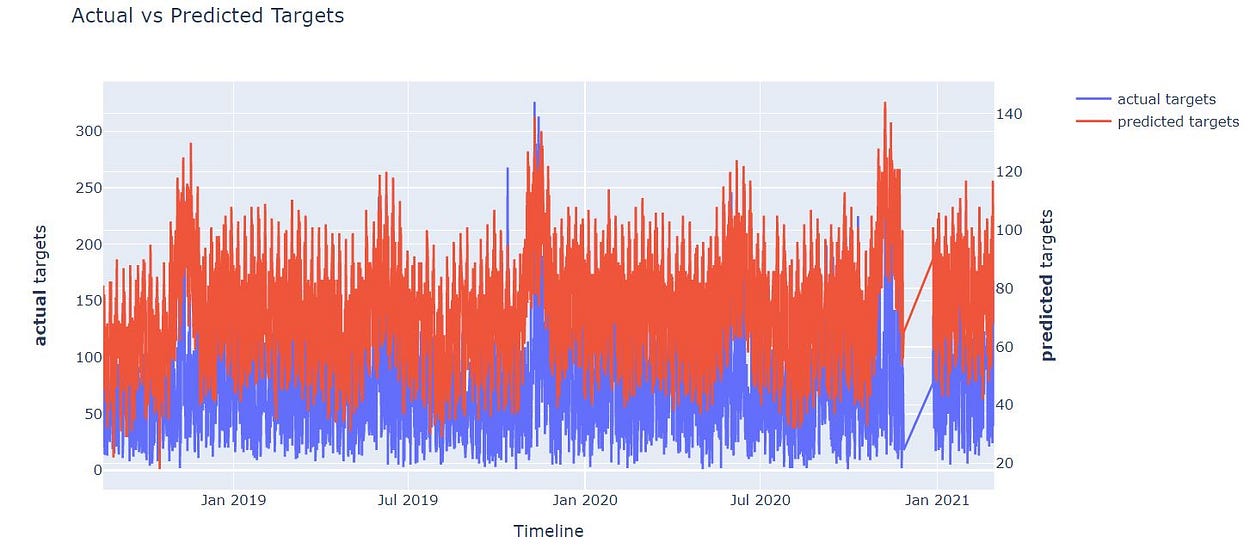
Note that the predicted values have some seasonality, and our predicted values explain that. The result given by the Prophet can be easily tweaked using parameters as well. For more details on tweaking, refer to this link.
Inference Phase
In the Inference Phase, we forecast the future values at some time intervals.
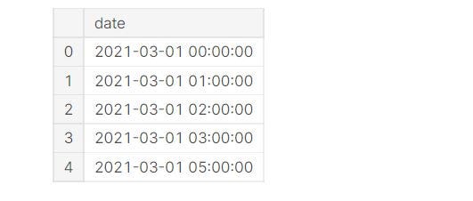
Here we have a test CSV file containing date and hour columns. The demand column is missing since we have to predict the demand.
test_data = pandas.read_csv('../input/jobathon-april-2022/test_6QvDdzb.csv')
print(f'test dataset size : {test_data.shape}')
testing_data = dataPreprocessing(test_data.copy())
testing_data.head()
We processed the data the same as we did for the training data. Our test data only contains the ds column, and the job is to predict the y column.
Note: Prophet models only understand the ds and y as input and output features. So before training and prediction, make sure we have renamed our columns.
test_prediction = model.predict(pd.DataFrame({'ds':testing_data['date']}))
Generating the Prediction
After Preparing the testing data, it’s time to call the prediction using prophet.
We add the demand column to our test data and assign the predicted values.
test_prediction = test_prediction['yhat']
test_prediction = test_prediction.astype(int)
test_data['demand'] = test_prediction
test_data.head()
test_data.to_csv('submission.csv', index=False)
Conclusion on Time Series Forecasting
In this article, we talked about the most straightforward implementation of time series analysis using the Facebook prophet library, and we used the Analytics Vidhya Jonathon April dataset.
- Time series analysis can be solved as a regression if it contains multiple columns ( Multi-variate time series forecasting)
- We can tweak the Prophet library by modifying the changepoints and other FB prophet parameters.
- Ensemble techniques can be used for time series analysis.
I hope you enjoyed reading this article. Here is my Linkedin link. Do connect with me.
The media shown in this article is not owned by Analytics Vidhya and is used at the Author’s discretion.


Since this is time series data, I believe we cannot split the data in a random fashion using train_data = training_data.sample(frac=0.8, random_state=10) as this will lead to data leakage. Thoughts?