Complete Flow of Decision Tree Algorithm
This article was published as a part of the Data Science Blogathon.
Introduction
In Machine Learning, there are two types of algorithms. One is Supervised, and the other is Unsupervised algorithms. A decision tree algorithm is a supervised Machine Learning Algorithm. There are many algorithms in supervised Machine Learning Algorithms like Random Forest, K-nearest neighbour, Naive Bayes, Logistic Regression, Linear Regression, Boosting algorithms, etc. These algorithms are used for predicting the output. Based on historical data, it will indicate the new output for new data. In detail will see below.
What is a Decision Tree Algorithm?
It is a Supervised Machine Learning Algorithm used for both classification and regression problems but primarily for classification models. It is a tree-structured classifier consisting of Root nodes, Leaf nodes, Branch trees, parent nodes, and child nodes. These will helps to predict the output.
Root node: It represents the entire population.
The leaf node represents the last node, nothing but the output label.
Branch tree: A subsection of the entire tree is called a Branch tree.
Parent node: A node, which is divided into sub-nodes, is called a parent node.
Child nodes: sub-nodes of the parent node are called child nodes.
Splitting: It is a process of dividing the node into subnodes is called splitting.
Pruning: It is a process of stopping the sub-nodes of a decision node is called Pruning. Simply, opposite process of splitting.
Decision Node: Splitting of a sub-node into further sub-nodes based on conditions is called Decision Nodes.
Working on Decision Tree Algorithm
In a decision tree, for predicting the class of the given dataset, the algorithm starts from the root node of the tree, and the decision tree algorithm compares the values of the root attribute with the record (real dataset) attribute and, based on the comparison, follows the branch and jumps to the next node. The algorithm again compares the attribute value with the other sub-nodes for the next node and moves further. It continues the process until it reaches the leaf node of the tree. The complete process can be better understood using the below algorithm:
Step-1: Select the root node based on the information gained value from the complete dataset.
Step-2: Divide the root node into sub-nodes based on information gain and entropy values.
Step-3: Continue this process till we cannot further classify the node into sub-nodes called leaf nodes.
An elementary example uses titanic data set for predicting whether a passenger will survive or not survive. I have used only three Columns/attributes/features for this example—namely, Sex, age, and sibs(number of spouses or children).
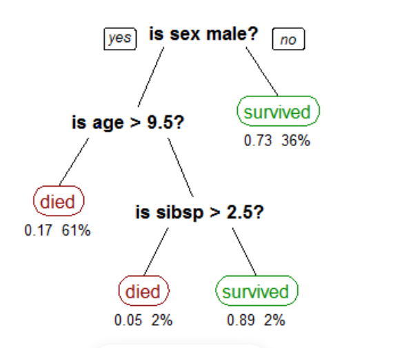
In the above figure, is sex male a root node? It will divide into two sub-nodes based on condition(yes or no). Is age>9.5?, is branch node and survived is Leaf node. Is sibsp>2.5?, is also a branch node, and died is a Leaf node. Both died and survived are Leaf nodes; there is no chance to split. In real datasets, there are more columns/attributes/features.
Implementing the Decision Tree Algorithm
While implementing the decision tree algorithm, everyone will doubt how to select the Root node and sub-nodes. We have a technique called ASM(Attributes Selection Measures). In this technique, there are two methods:
1. Information Gain:
2. Gini Index
Information Gain
entropy: It is the sum of the probability of each label times, the log probability of that same label. It is an average rate at which a stochastic data source produces information, Or it measures the uncertainty associated with a random variable.
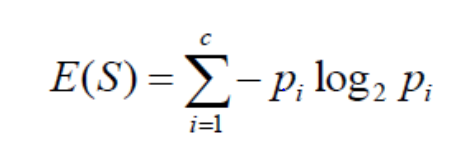

Where S=Total number of samples
P(yes)=Probability of Yes
P(No)=Probability of No
information Gain: An amount of information gained about a random variable or signal from observing another random variable.
It favours smaller partitions with distinct values.

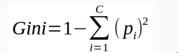
Gini Index
It is calculated by subtracting the sum of the squared probabilities of each class from one.
It favours larger partitions.
Decision Tree Algorithm: Pruning
In the tree algorithm, the Pruning concept will play a significant role. We may get the model overfitting issue when a model builds on a large dataset. For reducing this issue, Pruning will help.
Pruning is the process to stop the splitting of nodes into sub-nodes.
In this, there are two types:
1. Cost Complexity Pruning
2. Reduced Error Pruning
Implementation of Decision Tree Algorithm
For building a model, we need to preprocess the data, Transform the data, split the data into train and test, and then make the model.
Firstly, we need to import the dataset, assign it to a variable, and then view it.
import pandas as pd
import numpy as np
data=pd.read_csv('train.csv')
data.head()
Output:-
| Survived | Pclass | Sex | Age | SibSp | |
|---|---|---|---|---|---|
| 0 | 0 | 3 | male | 22.0 | 1 |
| 1 | 1 | 1 | female | 38.0 | 1 |
| 2 | 1 | 3 | female | 26.0 | 0 |
| 3 | 1 | 1 | female | 35.0 | 1 |
| 4 | 0 | 3 | male | 35.0 | 0 |
The Survived column is the output variable from the above image, and the remaining columns are input variables.
Next, we can describe the dataset and check the mean, standard deviation, and percentile values.
data.describe()
Output:-
| Survived | Pclass | Age | SibSp | |
|---|---|---|---|---|
| count | 891.000000 | 891.000000 | 714.000000 | 891.000000 |
| mean | 0.383838 | 2.308642 | 29.699118 | 0.523008 |
| std | 0.486592 | 0.836071 | 14.526497 | 1.102743 |
| min | 0.000000 | 1.000000 | 0.420000 | 0.000000 |
| 25% | 0.000000 | 2.000000 | 20.125000 | 0.000000 |
| 50% | 0.000000 | 3.000000 | 28.000000 | 0.000000 |
| 75% | 1.000000 | 3.000000 | 38.000000 | 1.000000 |
| max | 1.000000 | 3.000000 | 80.000000 | 8.000000 |
Preprocessing the Data
Check the missing values, whether is there any or not. If there, then replace it with mean or median or drop.
data.isna().sum()
Output:-
Survived      0
Pclass        0
Sex           0
Age         177
SibSp         0
dtype: int64
From the above image, 0 means no missing values present in the column, and 177 points 177 missing values current in that column. So, as of now, I removed the entire rows where missing values will be Present.
data.dropna(inplace=True)
After removing the missing values, rows then check once whether it was removed or not.
data.isna().sum()
Output:-
Survived    0
Pclass      0
Sex         0
Age         0
SibSp       0
dtype: int64
By seeing the above image missing values, rows are removed successfully.
The model only deals with Numerical data. So now check whether any categorical data will be present in the dataset. If any categorical attributes are present in input data, convert them into numerical points using dummy variables.
data.info()
Output:-
Int64Index: 714 entries, 0 to 890
Data columns (total 5 columns):
 #   Column    Non-Null Count  Dtype
---  ------    --------------  -----
 0   Survived  714 non-null    int64
 1   Pclass    714 non-null    int64
 2   Sex       714 non-null    object
 3   Age       714 non-null    float64
 4   SibSp     714 non-null    int64
dtypes: float64(1), int64(3), object(1)
memory usage: 33.5+ KB
In the above image, the Dtype object is present, which means that the Sex column is categorical. Now apply the dummy variable method and convert it to numerical.
data_1=pd.get_dummies(data.Sex,drop_first=True)
data_1.head()
Output:-
| male | |
|---|---|
| 0 | 1 |
| 1 | 0 |
| 2 | 0 |
| 3 | 0 |
| 4 | 1 |
Let’s see the above image, converting the sex categorical column into numerical. ‘1’ represents male, and ‘0’ represents female. As of now, I have not changed the male column name. If you want, you can. And now, remove the original column from the dataset and add the new column to it.
data.drop(['Sex'],inplace=True,axis=1)
data.head(3)
Output:-
| Survived | Pclass | Age | tbsp | |
|---|---|---|---|---|
| 0 | 0 | 3 | 22.0 | 1 |
| 1 | 1 | 1 | 38.0 | 1 |
| 2 | 1 | 3 | 26.0 | 0 |
data1=pd.concat([data,data_1],axis=1)
data1.head(3)
Output:-
| Survived | Pclass | Age | tbsp | male | |
|---|---|---|---|---|---|
| 0 | 0 | 3 | 22.0 | 1 | 1 |
| 1 | 1 | 1 | 38.0 | 1 | 0 |
| 2 | 1 | 3 | 26.0 | 0 | 0 |
See the above image new column will be added. Now all columns will be numerical.
Splitting the Data
Before splitting the data, First, divide the input and output data separately. Split the dataset into two parts training and testing with some ratio. When a model suffers from a fitting problem, then adjust the ratio.
y=data1[['Survived']]
y.head(2)
Output:-
| Survived | |
|---|---|
| 0 | 0 |
| 1 | 1 |
x=data1.drop([‘Survived’],axis=1)
x.head(2)
Output:-
| Pclass | Age | SibSp | male | |
|---|---|---|---|---|
| 0 | 3 | 22.0 | 1 | 1 |
| 1 | 1 | 38.0 | 1 | 0 |
from sklearn.model_selection import train_test_split
x_train, x_test, y_train, y_test= train_test_split(x, y, test_size= 0.30, random_state=0)
Let’s see the above image, x is the input variable, and y is the output variable. For both data, we imported the train_test_split method. We divided the data into 70:30 ratio means training data is 70%, and testing data is 30%. For that, we have given test_size=0.30.
Apply Transformation
Apply Normalization or standardization to bring all attributes values to 0-1. This will helps to reduce the variance effect.
from sklearn.preprocessing import StandardScaler
st_x= StandardScaler()
x_train= st_x.fit_transform(x_train)
x_test= st_x.fit_transform(x_test)
print(x_train[1])
print(x_test[1])
Output:-
array([-0.29658278, 0.10654022, -0.55031787, 0.75771531])
array([-1.42442296, 1.34921876, -0.56156739, -1.31206669])
From the above image, we can observe that all values are standardized.
Model Building
From the Sklearn library, import the model and build it.
from sklearn.tree import DecisionTreeClassifier
classifier= DecisionTreeClassifier(criterion='entropy', random_state=0)
classifier.fit(x_train, y_train)
Output:-
DecisionTreeClassifier(criterion='entropy', random_state=0)
By seeing the above image, I successfully built the model. This model has been created on training data.
Predict the Results
After building the model, we can predict the output.
y_pred= classifier.predict(x_test)
y_pred
Output:-
array([0, 1, 1, 0, 1, 0, 0, 0, 0, 0, 0, 0, 1, 0, 1, 1, 0, 0, 0, 0, 0, 1,
       1, 0, 0, 0, 1, 0, 1, 0, 0, 0, 0, 1, 0, 0, 1, 1, 0, 0, 0, 0, 0, 0,
       1, 1, 0, 0, 0, 0, 0, 1, 0, 1, 1, 0, 1, 0, 0, 0, 0, 0, 1, 0, 1, 0,
       1, 0, 1, 0, 0, 0, 1, 1, 1, 1, 0, 0, 0, 0, 1, 1, 1, 1, 1, 0, 0, 1,
       1, 0, 1, 0, 1, 0, 1, 0, 1, 0, 0, 0, 0, 0, 0, 1, 1, 1, 1, 1, 1, 0,
       0, 0, 0, 0, 0, 0, 0, 0, 1, 1, 0, 0, 0, 1, 1, 1, 1, 0, 0, 1, 1, 0,
       1, 1, 1, 0, 1, 0, 0, 0, 1, 0, 1, 1, 0, 0, 1, 0, 0, 0, 0, 0, 0, 0,
       0, 0, 1, 0, 0, 0, 0, 0, 0, 0, 0, 1, 1, 0, 0, 0, 1, 1, 1, 0, 0, 0,
       1, 0, 0, 1, 0, 0, 0, 1, 0, 1, 0, 1, 1, 0, 0, 0, 0, 0, 0, 0, 0, 1,
       0, 0, 1, 0, 1, 0, 0, 1, 0, 0, 0, 0, 0, 0, 0, 1, 0], dtype=int64)
Model built on training data and the prediction made on testing data. So, x_test was provided, For prediction, and it will predict the output of the x_train data.
Check the Accuracy
After predicting the output, For x_test, we can check with y_test and y_pred at what percentage of accuracy it will Predict.
from sklearn.metrics import confusion_matrix
cm= confusion_matrix(y_test, y_pred)
cm
Output:-
array([[106,  19],
       [ 32,  58]], dtype=int64)
The above image shows the confusion matrix of y_test and y_pred. We can calculate all the metrics like accuracy score, recall, precision, and sensitivity from this.
Conclusion
The decision tree algorithm is a supervised machine learning algorithm where data is continuously divided at each row based on specific rules until the outcome is generated. It works for both classification and regression models.
Decision tree algorithms deal with complex datasets and can be pruned if necessary to avoid overfitting. This algorithm is not suited for imbalanced datasets. This algorithm is more prevalent in the health, finance, and technology sectors.
Now that you have learned the basics, We will cover some practical applications of decision trees in more detail in future posts.
If you have any queries, content with me on LinkedIn
Read the latest articles on our blog.
The media shown in this article is not owned by Analytics Vidhya and is used at the Author’s discretion.


