Gain Customer’s Confidence in ML Model Predictions
This article was published as a part of the Data Science Blogathon.
Introduction
One of the key challenges in Machine Learning Model is the explainability of the ML Model that we are building. In general, ML Model is a Black Box. As Data scientists, we may understand the algorithm & statistical methods used behind the scene. But, when we show the outcome of the model to the customer, they may not understand all those technicalities & statistics. They will be primarily interested in understanding the different factors that influence the outcome (i.e., prediction done by ML Model).
For example: Let us say our ML model predicts the end customer who will subscribe to a particular banking product. When we show our ML Model result to our customers, their question could be, out of the given factors (dependent variables), which are the influencing factors & the values that will help us to decide whether a particular end customer will subscribe to a product or not.
It becomes a challenge to the data scientist to explain to the customer why a particular value is predicted by our ML model. We need to explain to the customer in a simple business language (without using technicality or statistics).
Explainable AI helps to overcome the above challenge.
Problem Statement
Let us take the Breast cancer dataset available from sklearn datasets. We can use this dataset to understand Explainable AI.
Breast cancer data contains 30 attributes & target class has two values (Malignant & Benign). Based on the patient’s test results, we need to determine whether it is Malignant or Benign. Doctors would be interested to understand which features & the associated values are helping us to predict the output using our Machine Learning Model.
Key Attributes of the Breast Cancer Dataset are Given Below
- Radius: Mean of distances from the center to points on the perimeter
- Texture: Standard deviation of grey-scale values
- Perimeter: Perimeter
- Area: Area
- Smoothness: Local variation in radius lengths
- Compactness: (Perimeter2 / Area) – 1.0
- Concavity: Severity of concave portions of the contour
- Concave points: Number of concave portions of the contour
- Symmetry: Symmetry
- Fractal dimension: “Coastline Approximation” – 1
Balance 20 attributes are the mean and the worst or largest value of the above features.
Let us read the data & load it. Post that extracts Input Data (Features) and target values.
from sklearn.datasets import load_breast_cancer as lbc
breast_cancer = lbc()
X = breast_cancer.data
y = breast_cancer.target
#Let us take target factor name and other input factor names. Also, get the number of input factors
target_name=breast_cancer.target_names
inp_features=breast_cancer.feature_names
num_inp_features=len(inp_features)
As per the below output, we have 569 records & 30 features in the breast cancer dataset.
print("Input Data Size : ", X.shape)
print("Target Data Size : ", y.shape)
Output:
Input Data Size : (569, 30)
Target Data Size : (569,)
Let us split the input data as Training and Validation sets:
from sklearn.model_selection import train_test_split
X_train, X_valid, y_train, y_valid = train_test_split(X, y, test_size=0.1, stratify=y, random_state=123)
Now we can build the ML Model using logistic regression. As this article primarily focuses on the Explainability of the ML model, we will build a simple model and fit the given data.
from sklearn.linear_model import LogisticRegression
log_reg=LogisticRegression(solver='liblinear')
log_reg.fit(X_train,y_train)
Explainable AI Method
We will use the LIME package. LIME stands for Local Interpretable Model-agnostic Explanations. It was developed by Marco Ribeiro in 2016. It helps in explaining predictions of Machine Learning models.
We need to pass our input data (X) and the feature names to the LimeTabularExplainer method.
#Let us import the lime_tabular
from lime import lime_tabular as lt
interpreter=lt.LimeTabularExplainer(
    training_data=X,
    feature_names=inp_features,
    class_names=target_name,
    mode='classification'
)
interpreter
Now let us look at the target value for the first few records from the validation dataset:
for i in range(15):
    print("Target Class for validation record-",i," is:",breast_cancer.target_names[y_valid[i]])
#Let us predict the output for our validation dataset using Logistic Regression ML model built.
y_pred=log_reg.predict(X_valid)
We can take one benign & one malignant record and use the Lime method to explain what features and values are used to determine respective predictions.
First, we can take the Malignant record.
idx=9
print("The Predicted value is: ", breast_cancer.target_names[y_pred[idx]])
print("The Actual value is: ", breast_cancer.target_names[y_valid[idx]])
explanation = interpreter.explain_instance(X_valid[idx], log_reg.predict_proba,
                                            num_features=num_inp_features)
#When we run the below command we will get the below image as an output
explanation.show_in_notebook()
The Predicted value is: malignant
The Actual value is: malignant
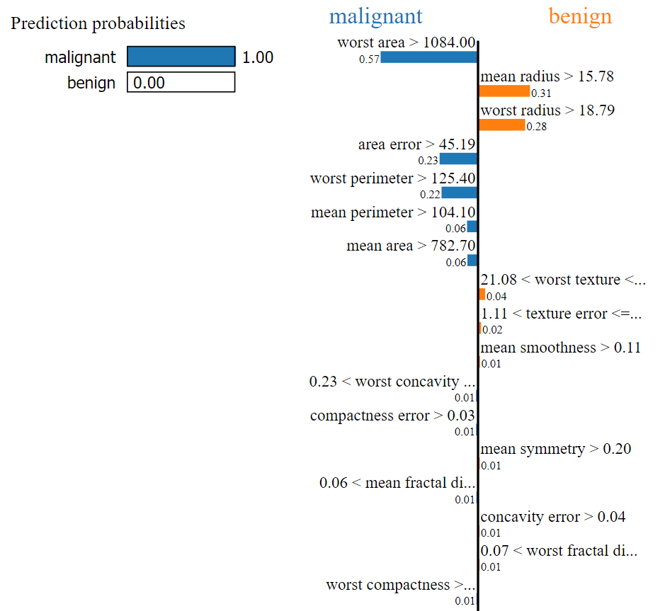
For this record, our ML model predicted the output as Malignant. By looking at the above image, we can easily determine that the values of the following factors helped to categorize our current test record as Malignant:
- Worst area
- Area error
- Worst perimeter
- Mean perimeter
- Mean area etc.
We can use the as_list method that returns the explanation as a list.
explanation.as_list()
[('worst area > 1084.00', -0.5743903734810332),

('mean radius > 15.78', 0.3065024565856821),

('worst radius > 18.79', 0.2781261572624384),

('area error > 45.19', -0.2266452607347196),

('worst perimeter > 125.40', -0.21512839211430862),

('mean perimeter > 104.10', -0.06480282417294424),

('mean area > 782.70', -0.062625153779533),

('21.08 < worst texture <= 25.41', 0.04189477470690242),

('1.11 < texture error <= 1.47', 0.018026672529532325),

('mean smoothness > 0.11', 0.011473814660395166),

('0.23 < worst concavity <= 0.38', -0.011362114163194194),

('compactness error > 0.03', -0.011128308511517988),

('mean symmetry > 0.20', 0.01014369342543094),

('0.06 < mean fractal dimension <= 0.07', -0.00951514079682355),

('concavity error > 0.04', 0.009128695176455334),

('0.07 < worst fractal dimension <= 0.08', 0.009086032236228479),

('worst compactness > 0.34', -0.009054490615474208),

('fractal dimension error > 0.00', 0.007132175789541012),

('mean concavity > 0.13', 0.006898706630114457),

('perimeter error > 3.36', -0.006723294106554326),

('worst symmetry <= 0.25', -0.0066812479443135045),

('mean concave points > 0.07', 0.006115692407880622),

('0.13 < worst smoothness <= 0.15', 0.004740877713944246),

('0.10 < worst concave points <= 0.16', 0.003072068608489919),

('18.84 < mean texture <= 21.80', -0.002912258623833895),

('0.02 < symmetry error <= 0.02', -0.002796066646601035),

('mean compactness > 0.13', 0.0024172799778361368),

('smoothness error > 0.01', 0.0007364097040019386),

('radius error > 0.48', -0.0006566959495514915),

('concave points error > 0.01', 1.7409565855185085e-05)]
Now we can easily determine that the predicted value will be malignant when
- worst area > 1084
- area error > 45.19
- worst perimeter > 125.40
- mean perimeter > 104.10
- mean area > 782.70
- 0.23 < worst concavity <= 0.38 etc.
Based on the below factors & given conditions, the predicted value will be benign.
- mean radius > 15.78
- worst radius > 18.79
- 21.08 < worst texture <= 25.41 etc.
In the above, the total weight* for Malignant is higher than the total weight of Benign, and it is predicted as Malignant.
* – In the as_list method output, weight is the second value in the tuple.
Now let us take another record where the actual target class is Benign.
idx=10
print("The Predicted value is: ", breast_cancer.target_names[y_pred[idx]])
print("The Actual value is: ", breast_cancer.target_names[y_valid[idx]])
explanation = interpreter.explain_instance(X_valid[idx], log_reg.predict_proba,
                                         num_features=num_inp_features)
#When we run the below command we will get the below image as an output
explanation.show_in_notebook()
The Predicted value is: benign
The Actual value is: benign
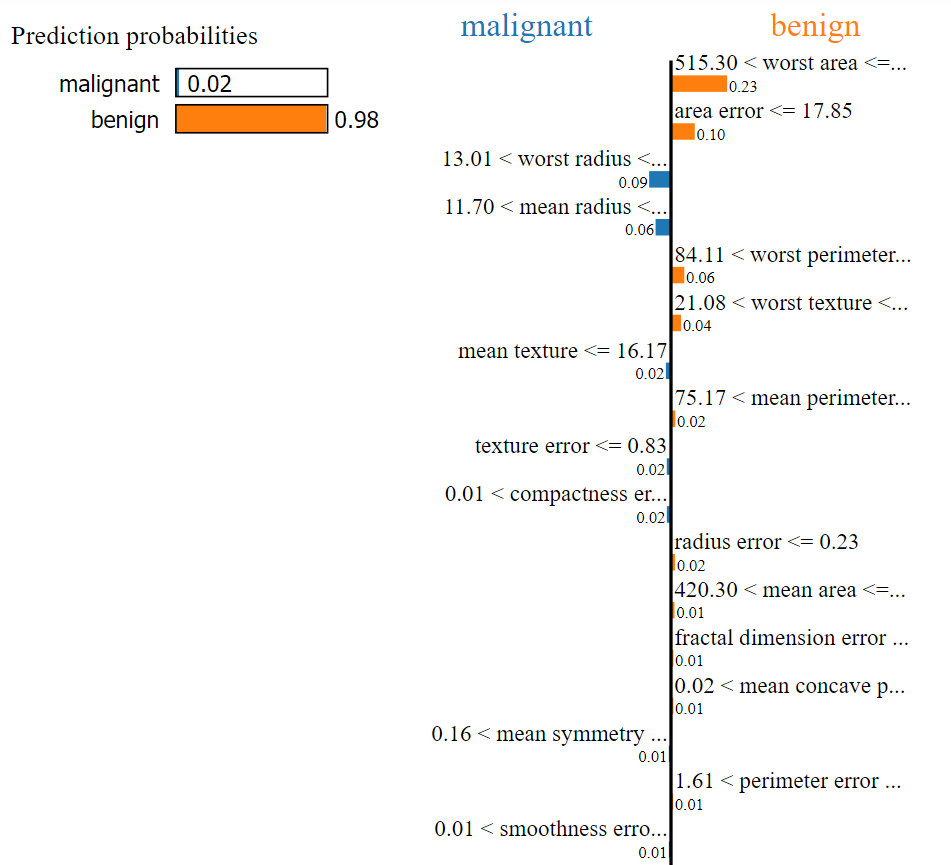
For this record, our ML model predicted the output as Benign. By looking at the above image, we can easily determine that the values of the following factors helped to categorize our current test record as Benign:
- Worst area
- Area error
- Worst perimeter
- Worst texture
- Mean perimeter etc.
We can use the as_list method that returns the explanation as a list.
explanation.as_list()
[('515.30 < worst area <= 686.50', 0.23423522343312397),

('area error <= 17.85', 0.09932481507185688),

('13.01 < worst radius <= 14.97', -0.0912969949900932),

('11.70 < mean radius <= 13.37', -0.06438274613297024),

('84.11 < worst perimeter <= 97.66', 0.05567602763452447),

('21.08 < worst texture <= 25.41', 0.04208188732942067),

('mean texture <= 16.17', -0.02136466132320542),

('75.17 < mean perimeter <= 86.24', 0.018076180494210392),

('texture error <= 0.83', -0.017610576785126807),

('0.01 < compactness error <= 0.02', -0.017351472875144505),

('radius error <= 0.23', 0.01676549847161827),

('420.30 < mean area <= 551.10', 0.014741343328811296),

('fractal dimension error <= 0.00', 0.01023889063543634),

('0.02 < mean concave points <= 0.03', 0.010054531003286822),

('0.16 < mean symmetry <= 0.18', -0.009116533387798486),

('1.61 < perimeter error <= 2.29', 0.00902644412074488),

('0.01 < smoothness error <= 0.01', -0.008978776136195118),

('0.09 < mean compactness <= 0.13', -0.008901319719466871),

('0.09 < mean smoothness <= 0.10', -0.008687995407606152),

('0.12 < worst smoothness <= 0.13', 0.008658688213409075),

('concave points error <= 0.01', 0.008212840751734897),

('0.03 < mean concavity <= 0.06', -0.00784969473029578),

('0.08 < worst fractal dimension <= 0.09', 0.0063961999268421854),

('0.02 < concavity error <= 0.03', -0.0059094106013907665),

('0.21 < worst compactness <= 0.34', 0.005438041960151277),

('0.10 < worst concave points <= 0.16', -0.004963081710033387),

('0.06 < mean fractal dimension <= 0.07', -0.003571533425273329),

('0.11 < worst concavity <= 0.23', 0.0015952771127532637),

('0.02 < symmetry error <= 0.02', 0.00020575600935763844),

('worst symmetry > 0.32', -2.4630829305295767e-06)]
Now we can easily determine that the predicted value will be benign when
- 515.30 < worst area <= 686.50
- area error <= 17.85
- 84.11 < worst perimeter <= 97.66
- 21.08 < worst texture <= 25.41
- 75.17 < mean perimeter <= 86.24
- radius error <= 0.23
- 420.30 < mean area <= 551.10 etc.
Based on the below factors & given the condition, the predicted value will be Malignant.
- 13.01 < worst radius <= 14.97
- 11.70 < mean radius <= 13.37
- mean texture <= 16.17 etc.
In the above, the total weight* for Benign is higher than the total weight of Malignant, and it is predicted as Benign.
* – In the as_list method output, weight is the second value in the tuple.
Let us take the Top 10 features from both of the above outcomes and take the union of them. As shown below, we will get14 features. We can build our ML model only with these Top Features alone and measure its performance.
Top10_Malignant_features = ['worst area','mean radius','worst radius','area error','worst perimeter','mean perimeter','worst texture','mean area','texture error','worst concavity']
Top10_Benign_features = ['worst area','worst perimeter','worst radius','mean radius','area error','worst smoothness','mean texture','worst concave points','mean symmetry','mean perimeter']
TopFeatures = list(set(Top10_Malignant_features).union(set(Top10_Benign_features)))
TopFeatures
Output:
[‘mean perimeter’,
‘mean symmetry’,
‘worst perimeter’,
‘worst texture’,
‘worst radius’,
‘area error’,
‘mean radius’,
‘worst smoothness’,
‘worst concave points’,
‘texture error’,
‘worst concavity’,
‘mean texture’,
‘mean area’,
‘worst area’]
For easy reading let us populate the above 14 features along with its condition in the below table.
| Malignant | Benign |
| [(‘worst area > 1084.00’, -0.5803518345205575) | [(‘515.30 < worst area <= 686.50’, 0.22554339363003018) |
| (‘mean radius > 15.78’, 0.3283066794435509) | (‘11.70 < mean radius <= 13.37’, -0.08990914134135829) |
| (‘worst radius > 18.79’, 0.2847121122126456) | (‘13.01 < worst radius <= 14.97’, -0.09756164435461571) |
| (‘area error > 45.19’, -0.19274455891418973) | (‘area error <= 17.85’, 0.0890550321024802) |
| (‘worst perimeter > 125.40’, -0.18712940680180037) | (‘84.11 < worst perimeter <= 97.66’, 0.1119793567357346) |
| (‘mean perimeter > 104.10’, -0.08673572096927613) | (‘75.17 < mean perimeter <= 86.24’, 0.026952609122275355) |
| (‘21.08 < worst texture <= 25.41’, 0.047850379213531656) | (‘21.08 < worst texture <= 25.41’, -0.003350298872178738) |
| (‘mean area > 782.70’, -0.03952532769795073) | (‘420.30 < mean area <= 551.10’, 0.025204070449238964) |
| (‘1.11 < texture error <= 1.47’, -0.02850008870427209) | (‘texture error <= 0.83’, -0.02330164946582758) |
| (‘0.23 < worst concavity <= 0.38’, 0.0273455173526529) | (‘0.11 < worst concavity <= 0.23’, 0.002536711602943987) |
| (‘0.13 < worst smoothness <= 0.15’, 0.015235108655295157) | (‘0.12 < worst smoothness <= 0.13’, -0.039083797050614585) |
| (‘18.84 < mean texture <= 21.80’, -0.005221933966127752) | (‘mean texture <= 16.17’, -0.03347715881547446) |
| (‘0.10 < worst concave points <= 0.16’, 0.011775720562469793) | (‘0.10 < worst concave points <= 0.16’, -0.0333650630221573) |
| (‘mean symmetry > 0.20’, -0.018969492633396663) | (‘0.16 < mean symmetry <= 0.18’, -0.027029769836097603) |
By looking at the above table, we can observe the following:
- For Malignant, the ‘worst area‘ value is > 1084. But for Benign, the ‘worst area’ value is between 515.30 and 686.50.
- For Malignant, the ‘mean radius‘ value is > 15.78. But for Benign, the ‘mean radius’ value is between 11.70 and 13.37.
- Same way, for Malignant, the ‘worst radius’ value is > 18.79. But for Benign, the ‘worst radius’ value is between 13.01 and 14.97.
- etc.
We could notice the differences in values for all of the above features between both of the classes.
- We can observe that the ‘worst texture’ value is between 21.08 and 25.41 for both of the classes.
- Same way, the ‘worst concave points’ value is between 0.10 and 0.16 for both of the classes.
- These features do not help us to distinguish the target classes.
Hence from the identified consolidated tp features, let us remove the above two features. Finally, we have a total of 12 Top Features.
TopFeatures.remove('worst texture')
TopFeatures.remove('worst concave points')
TopFeatures
Output:
Let us look at how many Malignant & Benign records are there in our overall & Validation Data set.
len(y[y==0]), y.sum()
len(y_valid[y_valid==0]), y_valid.sum()
Output:
In the overall dataset, we have 212 Malignant records and 357 Benign records. In the validation dataset, we have 21 Malignant records and 36 Benign records. Our target classes are not Balanced classes. Hence to measure the performance of our ML model, let us run the classification report.
from sklearn.metrics import classification_report
print("Classification Report for our Overall Validation Dataset is: ")
print(classification_report(y_valid, log_reg.predict(X_valid)))
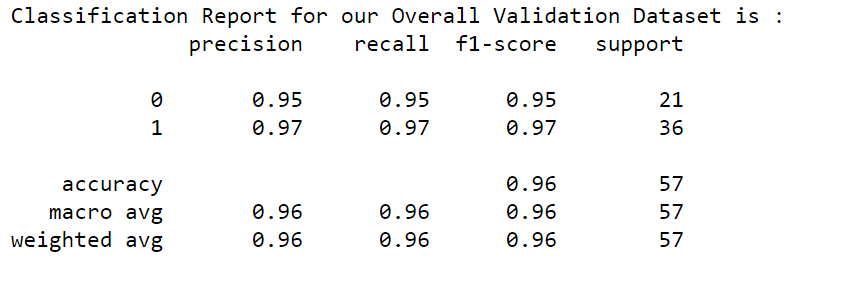
Our f1-score is 95% & 97% for both Malignant and Benign for our validation datasets with all 30 features.
Now, let us utilize the Top Identified features and pass those features alone to our ML model. Then run the Classification Report.
To do that let us create the dataframe for both Train and Validation datasets and while building the model pass the Top 12 Features alone.
import pandas as pd
X_train_df=pd.DataFrame(data=X_train,columns=inp_features)
X_valid_df=pd.DataFrame(data=X_valid,columns=inp_features)
log_reg_tuned=LogisticRegression(solver='liblinear')
log_reg_tuned.fit(X_train_df[TopFeatures],y_train)
y_pred_tuned=log_reg_tuned.predict(X_valid_df[TopFeatures])
print("Classification Report for our Validation Dataset with Top 12 Features alone is : ")
print(classification_report(y_valid, log_reg_tuned.predict(X_valid_df[TopFeatures])))
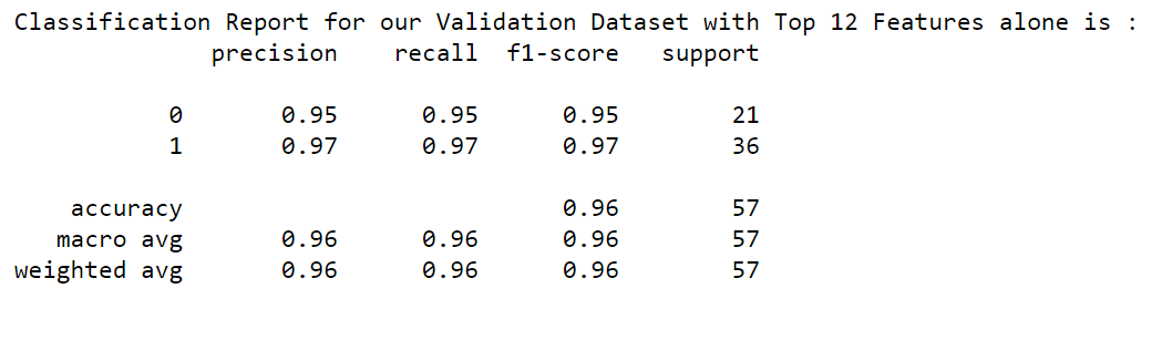
Wow!!! Our f1-score is 95% & 97% for both Malignant and Benign for our validation datasets with the selected Top 12 features. The performance of the model is retained at the same level.
Conclusion
As we discussed in the above article:
- Human believes other humans. Hence, if we share the Machine Learning model output with the customer, they may not get confidence in the predictions. They would like to see and understand what is happening behind the scene. But our ML Models are Black Box in nature.
- The LIME package helps us to open this Black Box Machine Learning model, and it explains the factors along with its values that are used to predict the outcome. Data scientists can use the output of the LIME package and provide simple explanations to the customer.
- It increases the confidence of our customers in the ML model that is built for them.
- We have also used the above output to identify the Top Features for both of the classes and passed those identified Top Features alone to the ML Model. We had observed that Model performance remained the same when we reduced the features from 30 to 12.
- So apart from using the LIME package to explain our ML Model to the customer, we saw how Data scientists could optimize the ML Model.
I hope you like this article. Kindly share your comments.
The media shown in this article is not owned by Analytics Vidhya and are used at the Author’s discretion.


