How to Convert Jupyter Notebook into ML Web App?
This article was published as a part of the Data Science Blogathon.
Introduction
Jupyter Notebook is a web-based interactive computing platform that many data scientists use for data wrangling, data visualization, and prototyping of their Machine Learning models. It is easy to use the platform, and we can do programming in many languages like Python, Julia, R, etc. By default, it comes with Ipython kernels, and if necessary, we can install other language kernels.
We’ll need more tools to see how our prototype model works in a production environment and how visualizations look in a dashboard because they can only be used to prototype models and do things like Data wrangling and Data Visualization. To do this, we must master new tools and devote effort to developing apps and dashboards. But what if we could turn our Jupyter notebook into an app without writing a single line of code? What if we could host such an app on a server and use it as a web app?
Mercury is a library that can convert your Jupyter notebooks into interactive web applications. In this article, we will see how to convert the Jupyter notebook into an application and deploy it on the Heroku platform.
Mercury
Mercury is an open-source library that can turn a jupyter notebook into a web application by just adding YAML parameters to the first cell of the notebook. It is developed by MLJAR Inc. There is a pro version of this with more features and support for a nominal price. You can find the documentation of this library at this link.

Building Application
We’ll use Random Forest to create a classification model on a Jupyter notebook, and then use Mercury to turn that notebook into an application by adding YAML parameters. This application will allow us to change the Random Forest algorithm’s hyperparameters and see the model’s results and charts for different hyperparameters. We’ll utilize the mushrooms dataset for this. Please use this URL to download the dataset.
Firstly we need to install the mercury library by using the following command.
pip install mljar-mercury
If you want to install using conda you can use the following command
conda install -c conda-forge mljar-mercury
Next, open the Jupyter notebook and we will import all the necessary libraries as shown below
import pandas as pd
import numpy as np
import matplotlib.pyplot as plt
from sklearn.ensemble import RandomForestClassifier
from sklearn.preprocessing import LabelEncoder
from sklearn.model_selection import train_test_split
from sklearn.metrics import plot_confusion_matrix, plot_roc_curve, plot_precision_recall_curve
from sklearn.metrics import precision_score, recall_score, accuracy_score
from termcolor import colored
import warnings
warnings.filterwarnings("ignore")
In the next cell, we create parameters for our Interactive web app and give default values as shown below
n_estimators = 100
max_depth = 1
bootstrap = 'True'
metrics_list = 'Confusion Matrix'
‘n_estimators’, ‘max_depth’, ‘bootstrap’ are hyperparameters that we will tweak and check for different evaluation metrics like accuracy, precision, recall. Also ‘metrics_list’ is a parameter that takes different plots like Confusion Matrix, ROC curve, Precision-Recall curve and plots them. Next, we load the dataset and create three functions namely ‘load_data()‘, ‘split(df)‘, ‘plot_metrics(metrcis_list)‘.
‘load_data()‘ function loads dataset and does label encoding.
‘split(df)‘ splits the dataset into training and testing datasets after separating the target column from the original dataset.
‘plot_metrics(metrics_list)‘ plots different metrics plots like Confusion Matrix, ROC Curve, and Precision-Recall curve. If you want more plots you can add them to this function.
We code the above functions as follows
data = pd.read_csv('mushroom.csv')
print(colored('Overview of Dataset', 'green', attrs=['bold']))
def load_data():
    label = LabelEncoder()
    for col in data.columns:
        data[col] = label.fit_transform(data[col])
    return data
def split(df):
    y = df.type
    x = df.drop(columns=['type'])
    x_train, x_test, y_train, y_test = train_test_split(x,y,test_size=0.3,random_state=0)
    return x_train, x_test, y_train, y_test
def plot_metrics(metrics_list):
        if 'Confusion Matrix' in metrics_list:
            plot_confusion_matrix(model, x_test, y_test, display_labels=class_names)
            plt.title("Confusion Matrix")
            plt.show()
        if 'ROC Curve' in metrics_list:
            plot_roc_curve(model, x_test, y_test)
            plt.title("ROC Curve")
            plt.show()
        if 'Precision-Recall Curve' in metrics_list:
            plot_precision_recall_curve(model, x_test, y_test)
            plt.title("Precision-Recall Curve")
            plt.show()
Now that we have loaded the dataset and coded all the required functions, let’s load the data and split it for training, and define class names as follows
df = load_data()
x_train, x_test, y_train,y_test = split(df)
class_names = ['edible', 'poisonous']
Now we create our Random Forest model, train it and get test predictions as follows
model = RandomForestClassifier(n_estimators=n_estimators, max_depth=max_depth,bootstrap=bootstrap,n_jobs=-1)
model.fit(x_train,y_train)
y_pred = model.predict(x_test)
In the next cell create a heading ‘Accuracy of the model’ and in the next cell code the following to get the accuracy
print("Accuracy: ", accuracy_score(y_test,y_pred).round(2))
Similarly, we do for ‘Precision score of the Model’, ‘Recall score of the Model’, and ‘Plot Metrics’ in separate cells
print("Precison: ", precision_score(y_test, y_pred, labels=class_names).round(2))
print("Recall: ",recall_score(y_test, y_pred, labels=class_names).round(2))
plot_metrics(metrics_list)
The above code gives the precision score, recall score of the model, and also it plots the different plots as per the input in the ‘plot_metrics‘ function.
So far we created things on the Jupyter notebook. Now, It’s time we convert our Jupyter notebook into an ML web app.
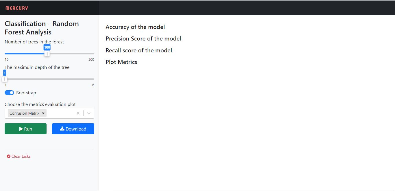
To do this we need to create YAML parameters in the first cell of the notebook. Go to the top of the notebook and insert a cell at the top and change the type of cell as ‘Raw NBConvert’. This is important. The type of this cell should be ‘Raw NBConvert’. Next, we create parameters for this web app as shown below
---
title: Classification - Random Forest Analysis
description: My first notebook in Mercury
show-code: False
params:
    n_estimators:
        label: Number of trees in the forest
        input: slider
        value: 100
        min: 10
        max: 200
    max_depth:
        label: The maximum depth of the tree
        input: slider
        value: 1
        min: 1
        max: 6
    bootstrap:
        label: Bootstrap
        input: checkbox
        value: True
    metrics_list:
        label: Choose the metrics evaluation plot
        input: select
        value: Confusion Matrix
        choices: [Confusion Matrix, ROC Curve, Precision-Recall Curve]
        multi: True
---
Here it is important to start with hyphens and end with hyphens as shown above. Apart from that, the allowed parameters in the YAML config are ‘title‘, ‘author‘, ‘description‘, ‘show-code‘, ‘show-prompt‘, ‘params‘. Also, there are different widgets available. For more on these please check this link and this link.
We define our parameters under ‘params‘ as shown above in the code. We can see each parameter has a ‘label‘ that gives the title of the widget. Next is we have ‘input‘ that gives the type of widget, then ‘value‘ that takes the parameter’s default value, and ‘min‘, ‘max‘ that defines the minimum and maximum value of the parameter.
So far we have created a prototype model in the jupyter notebook and added parameters in the YAML config. Now open the terminal to type the following code and run the mercury app on our device
mercury watch 'address of the notebook.ipynb'
This will open the application at this address ‘http://127.0.0.1:8000/app/1’. Or you can find all your mercury apps at this address ‘http://127.0.0.1:8000’.
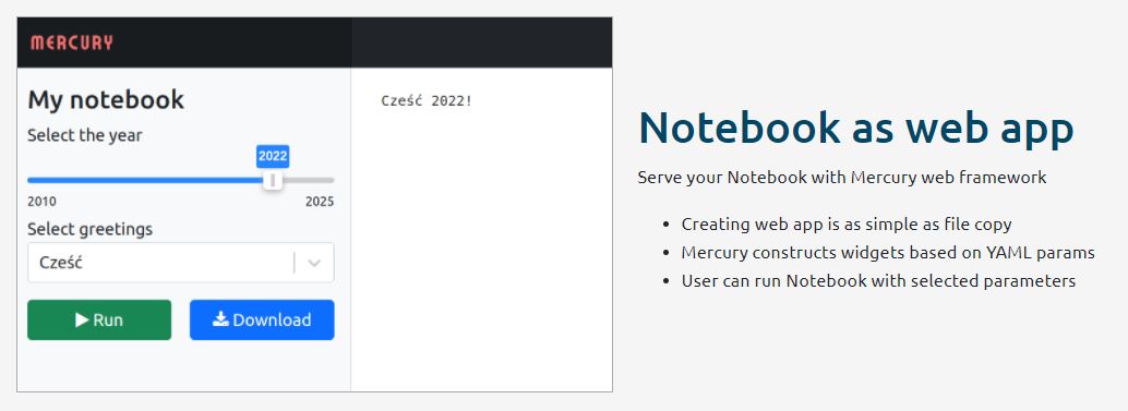
After you open your app, it will look something like this
Source: Mercury Share Python Notebooks
You can change the parameter values and click ‘Run’ to see the notebook displaying results. In this way, we can create a web app out of a jupyter notebook without using much code. We can create it just by adding some lines in the YAML config. Now that we have converted our Jupyter notebook into a Machine Learning Web application, let’s deploy it on Heroku so that we can access it anytime and just play with it by clicking the ‘Run’ button after tweaking the values.
Deploying on Heroku
We can deploy our application on Heroku. To do this, we have to create a ‘Procfile’, ‘requirements.txt’ file and upload the jupyter notebook, dataset file, and the two files we just created to Github.
So first, create a repo on Github and create a file with the name ‘Procfile’ and type the following and commit changes to it.
web: mercury run 0.0.0.0:$PORT
Next, create a file with the name ‘requirements.txt’ and type the following in that file and commit changes to it. This file is basically to tell Heroku what files to install to run our app.
mljar-mercury
matplotlib
scikit-learn
termcolor
ipython-genutils
pandas
numpy
Next upload the jupyter notebook we just created and the dataset that we used for this project.
Now create an account on Heroku if you don’t have one already and click ‘create new app’. Then follow the next steps and choose to connect the GitHub repo to deploy the app and click ‘Deploy’. Heroku will do the rest for us and gives us the link to our application. So finally we created our application and deployed it on Heroku.
The application I created is here Mercury (mercury-ml-web-app.herokuapp.com). You can open the link and check the application. You can create your application from a jupyter notebook in the way described above.
Conclusion
Thus, we had created an ML app from the jupyter notebook and deployed it on Heroku. Converting Jupyter notebooks into Web apps will make things easy and saves a lot of time. We can share jupyter notebooks in a convenient way and we can look at our prototype machine learning models in action in very less time. Mercury has made this job very easy for us without much code. Converting jupyter notebooks into web applications and sharing them online has become easy with Mercury.
Check out more examples from Mercury here Mercury (mljar.com)
The media shown in this article is not owned by Analytics Vidhya and are used at the Author’s discretion.


