Introduction to Probability Distributions for Data Science

This article was published as a part of the Data Science Blogathon.

Introduction to Probability Distributions

This article will focus on critical Probability Distributions from the data science point of view. We will divide these Probability distributions based on whether the data is discrete or continuous.

No matter what field you are in, Statistics and Probability will be there. Economics, Finance, Trading, Social sciences, Natural sciences and, of course, Data science is indispensable. A significant chunk of Data science is about understanding the behaviours and properties of variables, and this is not possible without knowing what distributions they belong to. Simply put, the probability distribution is a way to represent possible values a variable may take and their respective probability.

Discrete

• Bernoulli Distribution
• Binomial Distribution
• Poisson Distribution

Continuous

• Normal Distribution
• chi² Distribution
• Student-t Distribution
• Log-Normal Distribution
• Exponential Distribution

Density Functions

One of the critical things in any study related to distributions is Density functions. So, what are density functions? The density functions are mathematical functions that describe the probability distribution of a random variable X.

Probability Mass Function (PMF)

Probability Mass Functions describe the probability of a random variable X taking on a particular value x, and It is only applicable for discrete distributions. Mathematically PMF is given as

It must satisfy the below two conditions.

Probability Density Function (PDF)

The Probability Density Function is PMF equivalent but for continuous random variables. A continuous distribution is characterised by infinite numbers of the random variables, which means the probability of any random sample at a given point is infinitesimally low. So, a range of values is used to infer the likelihood of a random sample. And doing an integration over the range will fetch our likelihood for the same sample. Mathematically,

Cumulative Density Function (CDF)

A cumulative density function at x explains the probability of a random variable X taking on values less than or equal to x. It applies to distribution regardless of its type, continuous or discrete. For a constant distribution, all we need to do is integrate the density function from negative infinity to x.

And CDF for a random variable X sampled from a discrete distribution is given by

Finding the CDF of x is equal to the probability of random variable X <=x, which is, in turn, the summation of the possibility of X similar to x_i when x_i is less than or equal to x.

Discrete Distributions

As its name suggests, a Discrete Distribution is a distribution where observation can take only a finite number of values. For example, the rolling of a die can only have resulted from 1 to 6, or the gender of a species. It is fairly common to have discrete variables in a real-world data set, be it gender, age or visitors to a place at a particular time. There are a lot of other discrete distributions, but we will focus on the most common and important of them.

Bernoulli Distribution

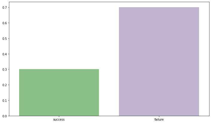
Bernoulli Distribution can be safely assumed to be the simplest 0f discrete distributions. Consider an example of flipping an unbiased coin. You either get a Head or a Tail. If we consider either of them as our priority(caring only about Head/Tail), the outcome will only be 0 (failure) or 1 (success). As it is an unbiased coin probability assigned to each outcome is 0.5. Remember, the outcome is always binary True/False, Head/Tail, Success/Failure etc.

The probability mass function or PMF of Bernoulli Distribution is given as

It can also be generalised as,

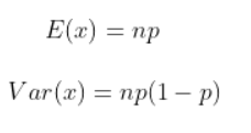
The expected value of the distribution can be derived by taking a weighted average of possible outcomes

and variance is given by

Cumulative distribution function

import seaborn as sns
import matplotlib.pyplot as plt
sns.set_palette('Accent')
fig,ax = plt.subplots(figsize=(12,7))
sns.barplot(y=[0.3,0.7], x = ['success','failure'],)

Binomial Distribution

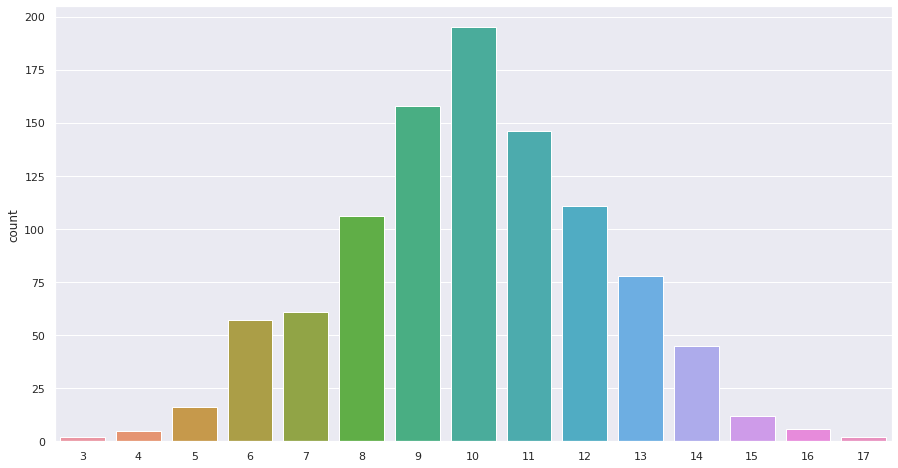
Binomial Distribution is simply an extension of Bernoulli distribution. If we repeat Bernoulli trials for n times, we will get a Binomial distribution. If we want to model the number of successes in n trials, we use Binomial Distribution. As each unit of Binomial is a Bernoulli trial, the outcome is always binary. The observations are independent of each other.

The Probability Mass Function is given by

where

and p is the probability of success

As binomial distribution is Bernoulli trials taken n number of times, the mean and variance are given by

The cumulative distribution function is given by

import numpy as np
import seaborn as sns
sns.set(style="darkgrid", palette="muted")
fig,ax = plt.subplots(figsize=(15,8))
binomial = np.random.binomial(20,0.5,1000)
sns.countplot(binomial)

Poisson Distribution

Poisson Distribution describes the probability of a given number of events occurring in a fixed interval, for example, the number of unique pageviews on an article on a given day or the number of customers visiting a florist shop at a particular time. It is not just limited to time intervals, and we can also extend its use to the area, length and volume intervals. For example, total rainfalls in a particular area.

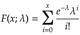
The Probability Mass Function for Poisson distribution is given by

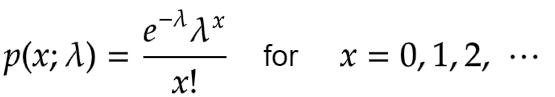
Here, lambda is the shape parameter that describes the average number of events in that interval.

lambda is also the mean and variance of the distribution.

The cumulative distribution function is given as

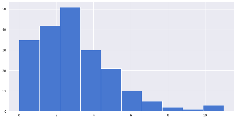
We will use scipy to simulate the Poisson distribution.

from scipy.stats import poisson
sns.set(style="darkgrid", palette="muted")
res = poisson.rvs(mu=3, size=200)
fig,ax = plt.subplots(figsize=(14,7))
plt.hist(x=res,)
plt.show()

Continuous Distributions

Continuous distributions, unlike discrete distributions, have smooth curves consisting of an infinite number of samples which means any random variable virtually can take any value. Weight, Height, stock prices, and the half-life of an object have continuous distributions. Unlike discrete statistical distributions, it is impossible to calculate the probability of a random variable equating to a certain value. For example, finding the probability that someone’s height is approximately 167cm is impossible. We are not talking about 167.0002 or 167.00001 but exact 167 cm, which is impossible to find in a continuous distribution. A range is used to find the probability of any value within the same range.

So, now let’s move on to our distributions.

Normal Distribution

The most common and naturally occurring distribution is Normal Distribution. It is otherwise also known as Gaussian Distribution. There is no field where this distribution is not seen. Finance, Statistics, Chemistry, you name it. It is an omnipresent distribution. A classic example could be the distribution of SAT scores higher number of students will score around the mean. As the distance increases from either side of the mean, the probability decreases.

The shape of the distribution resembles that of a classic bell, and hence it is called a bell-shaped curve. The curve is symmetric about its mean, and the variance defines the thickness of the distribution.

The mean, median and mode are the same in the case of Normal distribution.

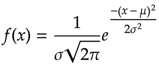
The Probability Distribution Function is given as

• Here, x = any random variable
• mu = mean
• sigma = standard deviation

When mu is 0 and variance/standard deviation is 1, it becomes Standard Normal Distribution.

The cumulative distribution function like we discussed, is the integral of PDF from negative infinity to the point for a standard normal distribution is given by

The Empirical Rule in normal distribution explains the probability of any random variable based on its standard deviation distance from the mean.

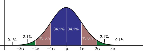
The probability of any random variable falling in the range of 1st std dev distance is 68% (either side). At the same time, the same for 2nd and 3rd std dev distance is 95% and 99%, respectively.

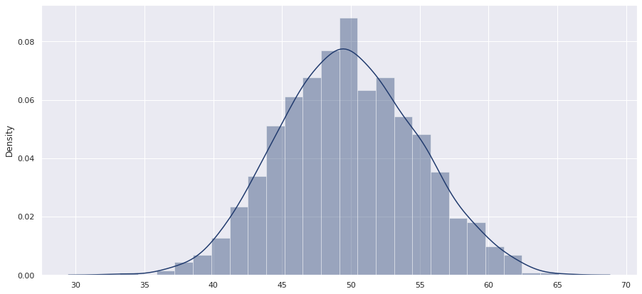
nums = np.random.normal(50, 5, 1000)
sns.set(style="darkgrid", palette="cividis",)
fig,ax = plt.subplots(figsize=(15,7))
sns.distplot(nums)

Chi² Distribution

A chi-square distribution can be defined as the distribution of the sum of the squares of v random variables drawn from a Gaussian or Normal distribution. The value v is also the degree of freedom of the distribution and the only parameter. For example, if 20 random variables are drawn from a normal distribution, the degree of freedom will be 20.

Unlike other distributions we have studied so far, the chi-square distribution doesn’t occur naturally. It is a theoretical distribution where the observations are calculated from the observations of a Normal distribution. The chi-square distribution is typically used in statistical significance testing where the underlying distribution is Normal.

The Probability Density Function is given by

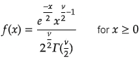
Where the capital letter gamma is the gamma function.

And the cumulative density function is given by

Here, the small letter gamma is the incomplete gamma function.

Thankfully, we have libraries to calculate all these and make our lives easier.

from scipy.stats import chi2
sample_space = np.arange(0, 20, 0.01)
dof = 2  #degree of freedom
pdf = chi2.pdf(sample_space, 2)
cdf = chi2.cdf(sample_space, 2)

import matplotlib.pyplot as plt
import numpy as np
from scipy.stats import chi2
import seaborn as sns
sample_space = np.arange(0, 20, 0.01)
sns.set(style="darkgrid", palette="muted")
fig,ax = plt.subplots(figsize=(15,7))
for dof in [1,2,3,4,5,6]:
  pdf = chi2.pdf(sample_space, dof)
  plt.ylim(0,0.4)
  sns.lineplot(x=sample_space, y = pdf, label= f'd0f = {dof}')
plt.show()

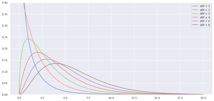
The more the degree of freedom, the more it appears Normal.

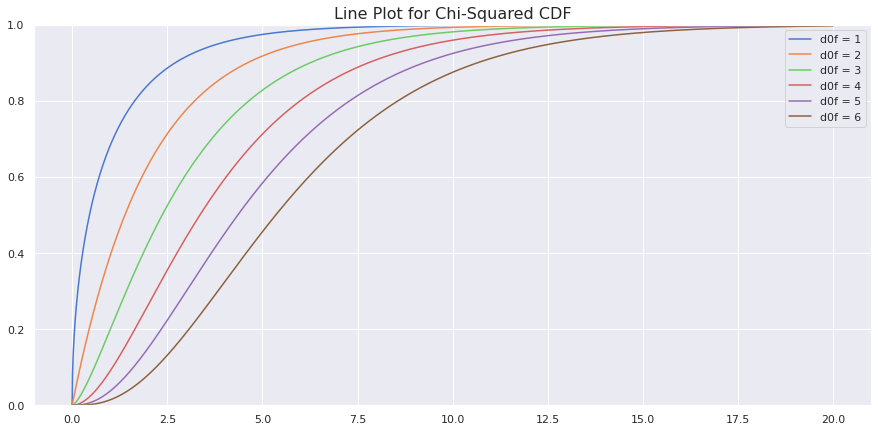
Plotting CDF

sample_space = np.arange(0, 20, 0.01)
sns.set(style="darkgrid", palette="muted")
fig,ax = plt.subplots(figsize=(15,7))
for dof in [1,2,3,4,5,6]:
  cdf = chi2.cdf(sample_space, dof)
  plt.ylim(0,1)
  sns.lineplot(x=sample_space, y = cdf, label= f'd0f = {dof}')
plt.title('Line Plot for Chi-Squared CDF',fontdict={'fontsize':16})
plt.show()

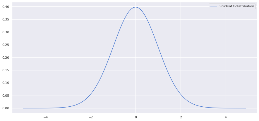
Student’s t-Distribution

In general, students’ t-distribution or t distribution is predominantly used in significance testing and construction of confidence intervals. Just as chi-squared distribution, t-distribution also doesn’t occur naturally. This distribution arises while estimating the mean of a normal distribution when the population parameters are unknown, and the sample size is relatively small.

The only parameter for t-distribution is the degree of freedom. If n is the number of samples drawn from a normal distribution, then the degree of freedom is n-1.

from scipy.stats import norm
from scipy.stats import t
sample_space = np.arange(-5, 5, 0.1)
dof = len(sample_space) - 1
fig,ax = plt.subplots(figsize=(15,7))
sns.lineplot(x = sample_space, y = t.pdf(sample_space,dof), label ='Student t-distribution')

 

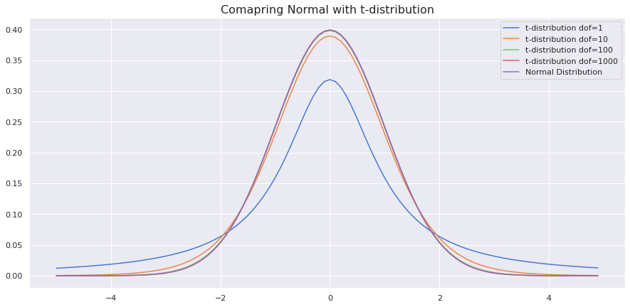
from scipy.stats import t
sample_space = np.arange(-5, 5, 0.1)
dof = len(sample_space) - 1
fig,ax = plt.subplots(figsize=(15,7))
sns.lineplot(x = sample_space, y = t.pdf(sample_space,1), label ='t-distribution dof=1')
sns.lineplot(x = sample_space, y = t.pdf(sample_space,10), label ='t-distribution dof=10')
sns.lineplot(x = sample_space, y = t.pdf(sample_space,100), label ='t-distribution dof=100')
sns.lineplot(x = sample_space, y = t.pdf(sample_space,1000), label ='t-distribution dof=1000')
sns.lineplot(x = sample_space, y = norm.pdf(sample_space,0,1), label = 'Normal Distribution')
plt.title('Comapring Normal with t-distribution', fontdict={'size':16})

Comparing CDF

from scipy.stats import t
sample_space = np.arange(-5, 5, 0.1)
dof = len(sample_space) - 1
fig,ax = plt.subplots(figsize=(15,7))
#t-sidtrribution plot
for  dof in [1,10,100,1000]:
  sns.lineplot(x = sample_space, y = t.cdf(sample_space,1), label =f't-distribution dof={dof}')
#normal distribution plot
sns.lineplot(x = sample_space, y = norm.cdf(sample_space,0,1), label = 'Normal Distribution')
plt.title('Comapring Normal with t-distribution', fontdict={'size':16})

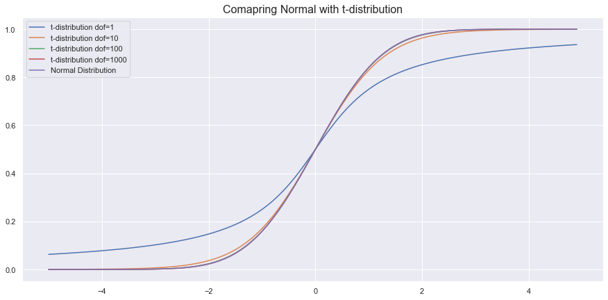
As we can see, as the degree of freedom increases, it resembles a normal distribution.

Log-Normal Distribution

The log-Normal distribution is a continuous distribution of random variables, whereas the natural logarithm of these random variables is a Normal distribution. So, if X is any log-normally distributed random variable, then ln(X) follows a Normal distribution. A Log-Normal distribution always yields positive values as opposed to Normal distribution. The log-normal distribution is used where we do not want to let go of the convenience of Normal Distribution yet want only positive outcomes. Height, Weight, Amount of milk production, Amount of rainfall etc., are cases where we can use the Log-Normal distribution.

The Probability Density Function is given by

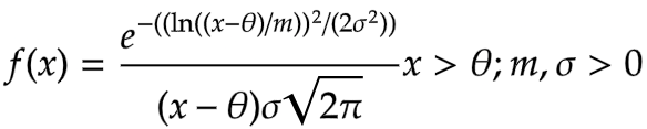
• here, the mu = location parameter tells about the location of the x-axis
• sigma = standard deviation
• m = the scale parameter responsible for shrinking of distributions
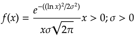
• When the theta=0 and m=1, it is called the Standard log-normal distribution.

When the theta = 0 and m = 1, it is called standard log-normal distribution.

The Cumulative Distribution Function is given as

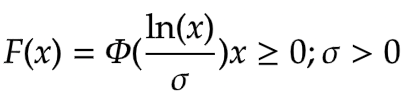
Where phi is the CDF of normal distribution

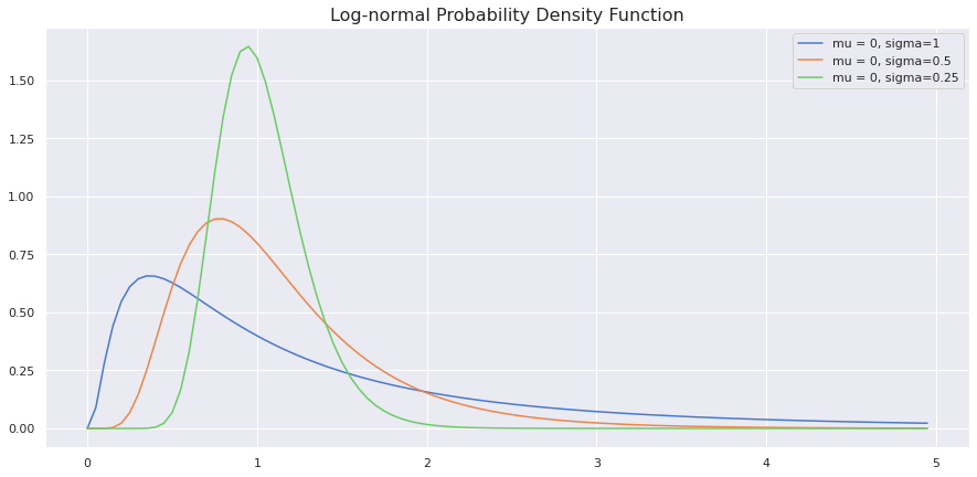
from scipy.stats import lognorm
sample_space = np.arange(0,5,0.05)
sns.set(style="darkgrid", palette="muted",)
fig,ax = plt.subplots(figsize=(15,7))
sns.lineplot(x=sample_space, y = lognorm.pdf(sample_space, 1,),
       label='mu = 0, sigma=1')
sns.lineplot(x = sample_space, y = lognorm.pdf(sample_space, 0.5,),
       label='mu = 0, sigma=0.5')
sns.lineplot(x = sample_space, y=lognorm.pdf(sample_space, 0.25,),
       label='mu = 0, sigma=0.25')
plt.title('Log-normal Probability Density Function',fontdict = {'size':16})

plt.plot()

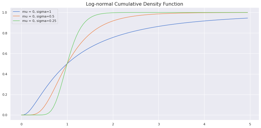
Cumulative Distribution Function

fig,ax = plt.subplots(figsize=(15,7))
sns.lineplot(x=sample_space, y = lognorm.cdf(sample_space, 1,),
       label='mu = 0, sigma=1')
sns.lineplot(x = sample_space, y = lognorm.cdf(sample_space, 0.5,),
       label='mu = 0, sigma=0.5')
sns.lineplot(x = sample_space, y=lognorm.cdf(sample_space, 0.25,),
       label='mu = 0, sigma=0.25')
plt.title('Log-normal Cumulative Density Function', fontdict = {'size':16})
plt.plot()

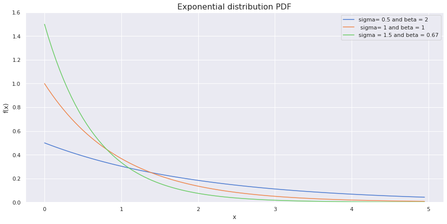
Exponential Distribution

The exponential distribution is often associated with the time elapsed until some event happens. The events within the time interval occur continuously and at an average constant rate. If you know high school chemistry, then chemical first-order reaction r time until a radioactive substance decays follow an exponential distribution. A more general example could be amount of months a car battery lasts.

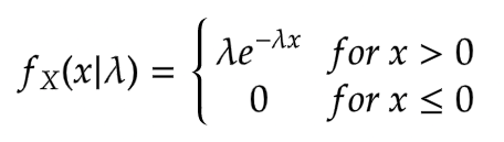
The general formula for PDF is

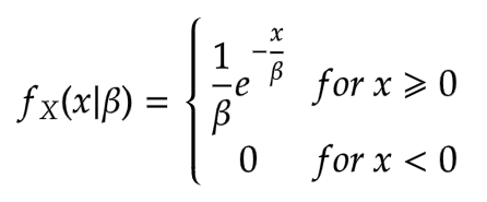
The pdf can also be parameterised with scale parameter beta, inversely related to lambda.

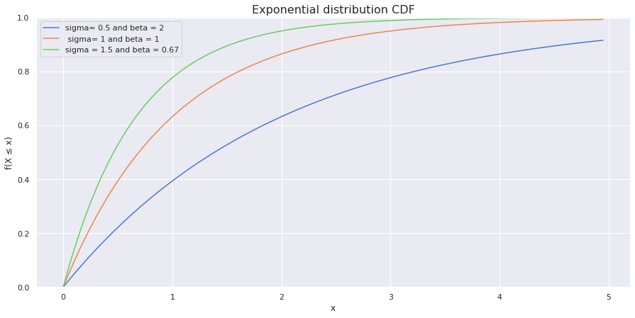
The CDF is given by

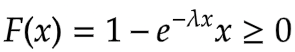
The same scale parameter can be substituted in place of lambda in the above CDF equation.

Here, the lambda is the rate of process change or called the rate parameter.

The mean and variance of the distribution are given by

from scipy.stats import expon
sample_space = np.arange(0,5,0.05)
sns.set(style="darkgrid", palette="muted",)
fig,ax = plt.subplots(figsize=(15,7))
plt.ylim(0,1.6,0.1)
sns.lineplot(x = sample_space, y = expon.pdf(sample_space,scale=2), label="sigma = 0.5 and beta = 2")
#scale parameter is used which is inverse of rate parameter
sns.lineplot(x = sample_space, y = expon.pdf(sample_space,scale=1), label="sigma = 1 and beta = 1")
sns.lineplot(x = sample_space, y = expon.pdf(sample_space,scale=2/3), label="sigma=1.5 and beta=0.67")
plt.ylabel('f(x)')
plt.xlabel('x')
plt.title('Exponential distribution PDF', fontdict = {'size':16})
plt.plot()

sample_space = np.arange(0,5,0.05)
sns.set(style="darkgrid", palette="muted",)
fig,ax = plt.subplots(figsize=(15,7))
plt.ylim(0,1,0.1)
sns.lineplot(x = sample_space, y = expon.cdf(sample_space,scale=2), label="sigma= 0.5 and beta = 2")
#scale parameter is used which is inverse of rate parameter
sns.lineplot(x = sample_space, y = expon.cdf(sample_space,scale=1), label=" sigma= 1 and beta = 1")
sns.lineplot(x = sample_space, y = expon.cdf(sample_space,scale=2/3), label="sigma=1.5 and beta=0.67")
plt.ylabel('f(X ≤ x)')
plt.xlabel('x')
plt.title('Exponential distribution CDF', fontdict = {'size':16})
plt.plot()

Conclusion on Probability Distributions

It is safe to say that statistics and Probability are precursors of Data science. And knowledge of Statistics and Probability to make better models is indeed essential. This article was a step in that direction. So, in this article.

• We discussed the properties of some of the required discrete and continuous statistical & Probability distributions.
• Learnt density functions of respective distributions along with formulas of means and variances.
• Finally, Python libraries (scipy, seaborn) were used to simulate and plot PDFs and CDFs of different distributions.

These are the essential distributions we observe in day to day data science tasks. There are some other distributions like Gamma and Beta, which could be important for some studies. Still, you will most likely encounter these distributions more frequently in your Data science journey.

The media shown in this article is not owned by Analytics Vidhya and is used at the Author’s discretion.

Sunil Kumar Dash 02 Jun 2022