All About Restaurant Recommender
This article was published as a part of the Data Science Blogathon.
Introduction on Restaurant Recommender
Now imagine the last time when you wished to order some clothes and what you were aware of is that you wish to get a shirt/top with polka dots as they were in fashion but once you are on amazon you struggle in finding the best design as there may be more than millions of polka dot pattern shirt in that case what you prefer is scrolling to recommended part and 40% of times you end up ordering items from recommended tabs.
So this problem accounts for major purchases in e-commerce and e-content-based apps, not just these 2 the list goes on and on.
This case study is built on datasets provided by www.akeedapp.com which is an online food delivery app based out of Muscat. It allows customers in Oman to order food from their favorite restaurants and have it delivered to their address. Datasets for this competition were made public here and this competition was closed on 16 August 2020.
The Competition was based on a supervised learning approach that is you were given with target that whether a customer is likely to order food from a vendor based on various information about both customers and vendors. But we will be using this as an unsupervised learning approach where we will be using all important data to figure out from where a customer can order his/her food which will save his time and effort and thus result in more food ordering.
Here we are given various CSV files each having specific values such as customers.csv is having values of approx 15500 different users which will be relevant to predict customer’s purchases, vendors.csv comprises 100 unique vendors that tell about vendor rating, products they cater to, and order.csv acts as joining table that can be used to join all csv files and create a new matrix.
Business Problem
=> Recommend vendors/restaurants to a consumer from which they are most likely to place an order
Flow Pipeline
Data preprocessing=> Feature creation=> Exploratory data analysis=> pose this problem as regression problem with order rating as target=> find feature important by tweaking a bit with features with like adding matrix completion features=> plot feature importance and take only those features which make significant impact => create a new matrix using only important factors and build user-user, vendor-vendor similarity=> predict most similar vendor with average rating more than 4 based on user-user similarity and vendor-vendor similarity
Error Metric
here as we pose this as a regression problem, therefore best metric that we can use is Root Mean Square Error (RMSE) which falls between (0-4). Root mean square is exactly as named, here xi is a true value whereas x^i is predicted value or model output and N here is the total number of rows in data set

1. Data Loading
you can download data from here. Data we will use consists of
- train_locations.csv – latitude and longitude for the different locations of each customer.
- train_customers.csv – details of each customer.
- orders.csv – orders that the customers train_customers.csv from made.
- vendors.csv – vendors that customers can order from.
Import this data to same folder where you will create your notebook. As you can see data here consists of 4 different files so we need to preprocess each file and join them based on their primary foreign keys, we will use the inner join method to merge all files based on customer_id and vendor_id from orders.csv.
2. Importing Libraries
import pandas as pd
import numpy as np
import matplotlib.pyplot as plt
import seaborn as sns
from datetime import datetime
from time import mktime
from xgboost import XGBRegressor, plot_importance
from sklearn.model_selection import train_test_split,GridSearchCV
from sklearn.metrics.pairwise import haversine_distances
from math import radians,sqrt
from tqdm import tqdm
from surprise import Reader, Dataset, BaselineOnly ,SVDpp, KNNBaseline
from tensorflow.test import gpu_device_name
import pickle
from sklearn.metrics import mean_squared_error,make_scorer
from statistics import mode
import warnings
warnings.filterwarnings('ignore')
3. Data Preprocessing
This is the important step as there are a lot of features that are not useful and have no importance by either having just one unique value or having so we need to eliminate them one by one starting with
Vendor.csv
vendors.csv file contains about 56 features and most of them are useless. we have to find useless features drop them, check if some features require some feature modification or up-gradation, and then replace all NaN values with the best substitute value based on their correspondence feature values.
Customers.csv
Customers.csv file contains about 8 features from which DOB, status, created_at, and updated_at are not useful as DOB is very sparse whereas status contains only 35 values with status=0 from 34674 value counts and this will end up affecting our end models. So it is better to remove also those rows where status = 0
Orders.csv
orders.csv contains 26 features but here we can see most people have rated 0 which is not possible, while deep-diving into our data we found that these were orders which were never rated which happens in real life so here for our discussed metric we need to remove all rows which were not rated and all those where rating given is 0
As delivery dates to most rows are null it cannot be used to define data as temporal in nature, whereas we can create a new feature time taken which is the time from which food is ordered to the time till which order is received by customers as most customers don’t care about what time it took to prepare and what time it took to deliver. They just care about once they ordered food, what time it takes for an app to deliver their order.
Now drop all useless feature that don’t add value that is order_accepted_time, driver_accepted_time, ready_for_pickup_time, delivered_time
Merging All to Create Final.csv
Create final data frame by joining vendors.csv, customers.csv on orders.csv using inner join method
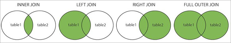
copyright https://www.softwaretestinghelp.com/inner-join-vs-outer-join/
Now apply haversine distance to find the geographic distance between customer location and vendor location here haversine distance may be a new term to many but it is a distance specific to geographic and drop customer location and vendor location
vendor_tag and vendor_tag_name are both the same and we can drop one from both so we would like to drop vendor tag and use vendor tag name to create a new feature and convert all customer_id from string integer
4. Exploratory Data Analysis
Here we try to figure out some useful data insights once we are done with all data cleaning and preprocessing as data processing is all about asking some good questions
What rating customer gives to restaurant on every order?
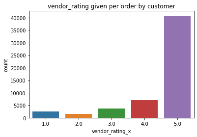
It shows either most users are biased towards giving good lenient ratings or most vendors are giving extremely good quality food
What does the past average rating per vendor look like?
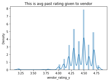
It also shows that most vendors are rated on average between 4.0 and 5 and no vendor is having rating less than 3
What is the delivery distance in KM for every order?
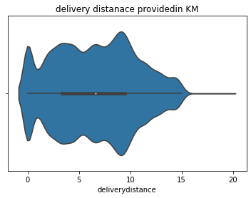
It shows that the median delivery distance lies near 6km with the 25th percentile near 3km and 75th percentile near 10km and most orders are delivered to about 10km
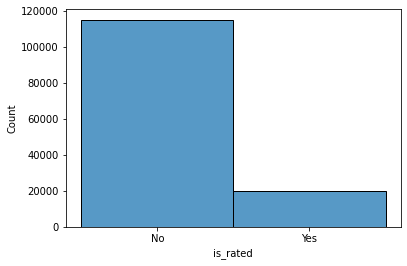
How many customers order food from their favorite restaurants or vendors?
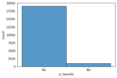
here we can see very less people order food from there favorite vendors
How many orders a customer place?
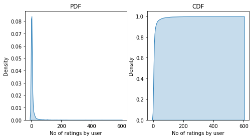
Here from both PDF and CDF, we can see that most users tend to place very few orders that are even less than 50 whereas some customers order more than 600 that is also possible is these may be bachelors or students who generally order food
How many orders each Restaurant is getting?
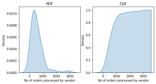
This turns out to be healthy competition mostly whereas only 10% of vendors are getting more than 1500 orders in a given time span
How many customers are placing an order from how many different restaurants?
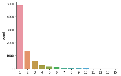
This shows that user voted for max 15 vendors and data looks healthy
5. Recommendation Systems
A recommendation system or recommender system is a type of information filtering system that uses various features given about user and product and tries to predict the most similar pairs to identify the best products according to user taste that a user is most likely to consume and return positive feedback. To apply this heavy-sounding technique what it uses at its heart is distance, understand it like a clustering thing where most similar techniques remain close to each other and as close 2 things are more are the chances that they end up being identical.
Recommender systems fall under 2 categories
1. Content Based Recommender System
This type of recommender system is useful for solving cold start problems. Here you use the past spending habits of a user and their past order details along with the past record of a vendor to track what rating they are most likely to give to that particular order this ultimately turns out to be one of our very familiar datasets type that is Regression. Here we can use our vendor rating per order as a target and rest other data as input and train a Regression model that helps us to predict what ratings user is going to give and based on that we can recommend those restaurants which tend to get a good rating or above 4 ratings.
2. Collaborative Filtering
This can be understood as similarities between 2 things whether it may be users or items. As they are just similarities they are not dependent on understanding data completely but they also arise with a problem of cold start that is whenever you are having a new user this method fails as you have no rating data about users.
User-User Collaborative Filtering
for example if customer 1 rates vendor 113, 71, 34 with 5 stars and customer 2 rates vendor 113, 40,71 and you know that customer 3 orders food and rates vendor 71 with 5 stars then there is a very high likelihood that he is going to rate vendor 113 with 5 stars ratings too. Here you can find how similar both users are using a similarity matrix which can be any but we are using cosine similarity here which is
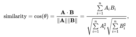

This is a very good gif that shows the depiction of user-user similarity here you can see the underlying question was whether a user will like a laptop based on his experience with a console, books, and some images
Item-Item Collaborative Filtering
This works on product-product similarity or in our case we can say restaurant-restaurant similarity based on how much time it takes to deliver food, items they offer average rating of vendor, and many more. all features that are not dependent are vendor dependent and this can be understood by example say customer 1 orders food from vendor 113 who provides them with shakes and smoothies along with a burger and he also orders food from vendor 40 who also provides shakes and beverages along with kinds of pasta then, in that case, there are very high chances that customer 1 wants to have some food along with shakes or smoothies every day so whenever we recommend him a customer we need to take care of drinks thing and recommend those restaurants which provide shakes along foods
6. Model Selection
From the discussion held above we know that we need a Regression model which can provide us back with feature importance as feature importance will be of use and as dimensions here are not too large we can go for gradient boosting algorithms or linear regression but while working with XGBRegression we need to take care about overfitting of our models as it may turn out to be a great problem also XGBRegression supports GPU training which helps us train our model faster.
With this discussion, we are convinced enough to go with XGBRegressor as our regression model
7. Hyper-parameter Tuning
We will be using grid search CV to get best hyper-parameter with xgboost and this can be done using in this we will use a self defined scoring function for RMSE score during our Grid Search cv operation with GPU enabled XGBoost algorithm
Now lets pass outcome of this snippet to our actual Regression
Here we will use output of function hyperparamter to best our best tunned model, then we will plot train vs test loss for each estimator an plot change in test RMSE and train RMSE that looks like
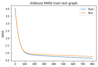
This can be used to detect weather a model is over fitting or not
now post tuning our model we will check distribution of RMSE after n estimators
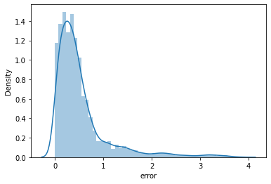
From this we can observe that most vakues have RMSE<0.5 which is positive for and we can use this to predict our data
8. Surprise library
Surprise library is built for recommender systems where it uses user, item, and rating to predict ratings for user-item interaction. for this, it implies various models like SVD, KNN matrix factorization, and many others that you can use to predict, and later you can use them as a feature and find changes in RMSE values
To apply the surprise library we need to initialize our data set as a trainset and testset
from surprise import Reader, Dataset
reader = Reader(rating_scale=(1,5))
# create the traindata from the dataframe...
train_data = Dataset.load_from_df(X_train[['customer_id', 'vendor_id', 'vendor_rating_x']], reader)
trainset = train_data.build_full_trainset()
#we are just adding both as we
testset = list(zip(X_test.customer_id.values, X_test.vendor_id.values, X_test.vendor_rating_x.values))
till here we created our train and test sets
Baseline Model

μ : Average of all trainings in training data.
bu : User bias
bi : Item bias (movie biases)
Here we train our model and save output rating to both train and test file
SVD Model

KNN
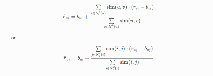
here first one is based on user-user metric where as second one is based on item-item metric
bui – Baseline prediction of (user,movie) rating
Nki(u) – Set of K similar users (neighbours) of user (u) who rated movie(i)
sim (u, v) – Similarity between users u and v
- Generally, it will be cosine similarity or Pearson correlation coefficient.
- But we use shrunk Pearson-baseline correlation coefficient, which is based on the pearson Baseline similarity ( we take base line predictions instead of mean rating of user/item)
9. Plotting Results
Now lets plot feature importance and obtain just some limited features which tends to have significant impact in our recommender systems
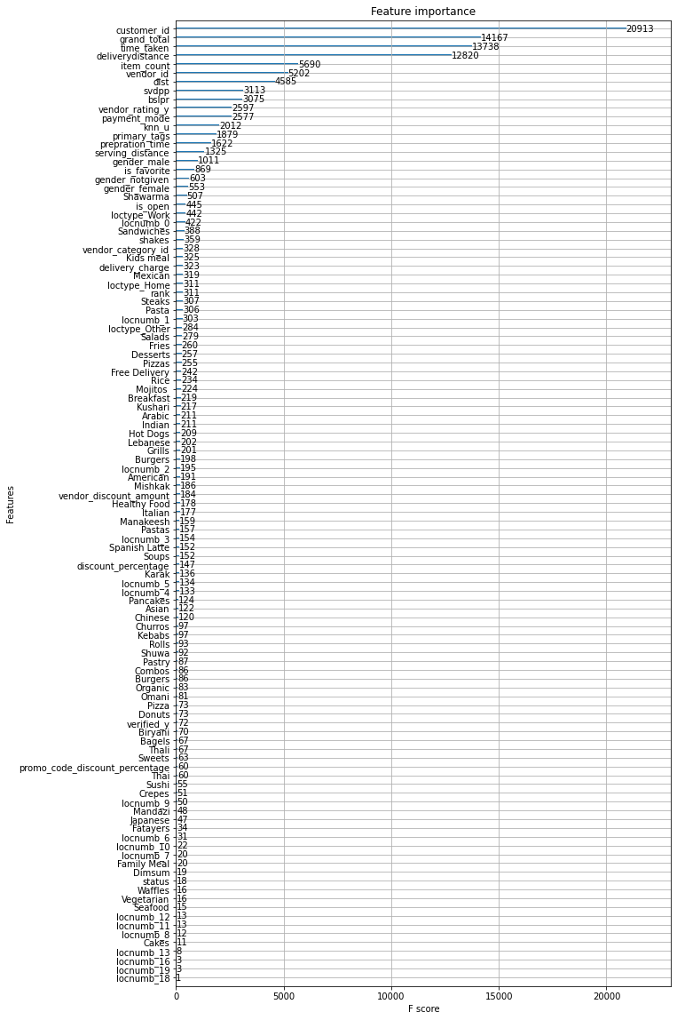
From here we can see that we can just use customer_id, grand_total, time_taken, deliverydistance,vendor_rating_y, vendor_id and pass that to a regression model
Adding outputs of each feature one by one to our train and test value and then obtaining the RMSE value for each regression model with different features we obtain
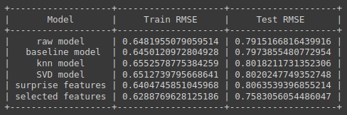
Here we can observe that models with very limited features tend to give good results over models with extra features this also clear a misconception of many that more dimensionality of data always tends to give better results
10. Collaborative Filtering-based Approach with Selected Features
Customer-customer Similarity
Now we will use features that were used in selected features to build a metrics by making all features standards and computing cosine similarity between each feature of each row and at last will use this to compute overall metrics
Vendor-vendor Similarity
Here we were given 100 different vendors and we will use selected features except both customer_id and vendor_id to get cosine similarity metrics between both
This can be done using
11. Testing
we can test our recommender system using
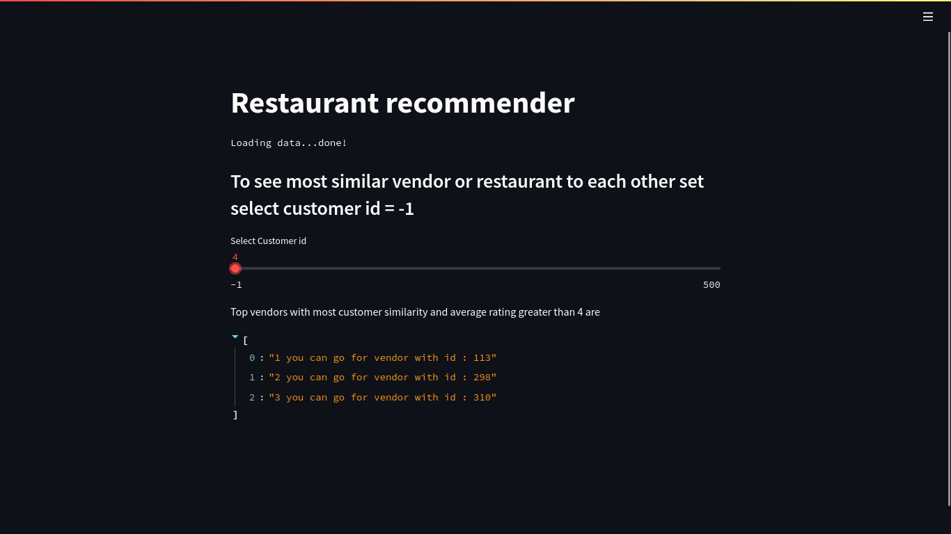
enter a customer id in range of 0-100
4
****************************************************************************************************
top recommended vendors are
****************************************************************************************************
1 you can go for vendor with id : 113
2 you can go for vendor with id : 298
3 you can go for vendor with id : 310
12. Deployment
To deploy this code we will use stream lit and heroku for deployment
Here we make a slider for customer id that lies in range of -1,1000 here if customer id is left to -1 than it enables recommend by vendor option and search for most similar vendors by vendor-vendor relation
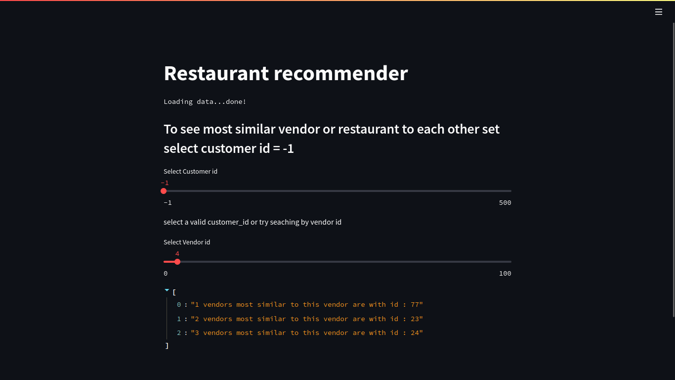
Else it works on customer customer similarity
Conclusion on Recommender
This case study discusses various approaches that can be used in process of building a conventional recommender system as we modified uses of this data set thus we cannot compare it with others. We also came to know that it’s not that more and more features are always good sometimes elimination of some features adds significant value to our models and this case study also discusses the approach of understanding a business first before solving a problem as without that we won’t be able to find that we need to remove 0 rating with high occurrence.
As the RMSE value curve shows that even if the mean is near 0.75 medians is below 0.5 which means there are extremely high chances of accurate recommendation also seeing our train test RMSE curve per epoch we know that neither our model is underfitting nor it is overfitting
We can use customer-customer similarity for the prediction with some selected parameters
Takeaways on Recommender
- We discussed various approaches to building a recommender system
- Feature removal can also lead to an increase in model performance
- Ways to convert recommender system problem to regression problem
- Learned to utilize surprise library to get new features
You can get ipython notebook from here
The media shown in this article is not owned by Analytics Vidhya and is used at the Author’s discretion.


how do you recommend new content to existing users using collaborative filtering?