All you Need to Know About AutoEncoders in 2024
This article was published as a part of the Data Science Blogathon.
Introduction
As the world develops rapidly with advances in machine learning and artificial intelligence, we will soon face a situation of uncontrollable data augmentation. GPUs, TPUs, and other faster storage and processing mechanisms have so far successfully processed vast amounts of data in the shortest possible time but can process data in less space. You also need to consider how to compress and store it. And that brings us to the topic of today’s discussion – autoencoders, a technique that allows us to compress available information.
Autoencoders are unsupervised learning techniques based on neural network frameworks, trained to copy inputs to outputs. Neural networks are designed to create bottlenecks in the network. Internally, the hidden layer h describes the code used to represent the input. An autoencoder network consists of three parts. First, the encoder compresses the image and generates code using the encoder function h = f(x). Then comes a bottleneck where we have a compressed knowledge representation of the original input, followed by a decoder that forms the reconstruction r = g(h). The autoencoder scheme is shown in Figure 1. Data is compressed and restructured as it moves through the architecture. This compression and reconstruction process is complicated when the input features are independent. However, if there is some correlation within the input data, the existing dependencies can be learned and used when the input is forced through the network bottleneck.
In the following subsection, we will take a detailed look into the network architecture and the corresponding hyperparameters of an Autoencoder.
The Architecture of an AutoEncoders
You must already have a faded idea of what an autoencoder would look like. In this section, we will add more depth to your understanding. We would be particularly interested in the hyperparameters you need to take care of while designing an autoencoder.
As mentioned earlier, an autoencoder consists of three parts: encoder, code, and decoder. Both the encoder and decoder are simple feedforward neural networks. The code is a single layer of ANN with selected dimensions. For input and output layers, the number of nodes is determined by the input data X. Therefore, the input and output layers have the same number of nodes, and both correspond to high-dimensional representations. The middle hidden layer with the fewest nodes corresponds to the low-dimensional representation. The goal of the training process is to minimize the squared reconstruction error between the network’s inputs and outputs. For learning algorithms, the most commonly used strategy is backpropagation. The initial weights of the network are important for the encoder to find a good solution. Backpropagation works more effectively when the initial weights are closer to the optimal solution. Many algorithms have been developed to find good initial weights.
Before training the autoencoder, we need to set four hyperparameters.
- The number of nodes in the middle layer, i.e., the code layer. A smaller size of the code layer would result in more compression.
- Then comes the number of layers in the encoder and decoder architectures. The depth of the architecture can be fine-tuned to perfection, and deep architecture has advantages over external networks.
- The number of nodes per layer is the third hyperparameter we need to tune. Typically the encoder and decoder are symmetric in terms of the layer structure, and the number of nodes in each subsequent layer of the encoder keeps decreasing till the code layer is reached and then keeps increasing similarly in the decoder architecture.
- The choice of the loss function is the fourth hyperparameter. The most frequently used loss functions include the mean squared error or binary cross entropy.
The most important tradeoff in autoencoders is the bias-variance tradeoff. At the same time, the autoencoder architecture should reconstruct the input well (reducing the reconstruction error) while generalizing the low representation to something meaningful. Therefore, to achieve this property, let’s look at the various architectures developed to address this trade-off.
Autoencoders types to tackle the tradeoff
1. Sparse Autoencoders
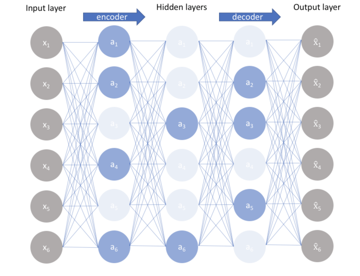
These networks offer an alternative method of introducing bottlenecks without requiring node count reduction. It handles the trade-off by forcing sparsity on hidden activations. They can be added over or in place of bottlenecks. There are two ways to apply sparse regularization. The first is by using L1 regularization, and the second is by implementing KL divergence. I won’t go into the mathematical details of the regularization technique, but a brief overview is sufficient for this blog.

Figure 2 – Schematic representation of a Sparse Autoencoder
2. Denoising Autoencoders
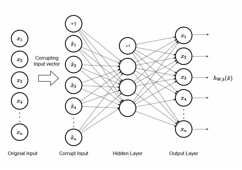
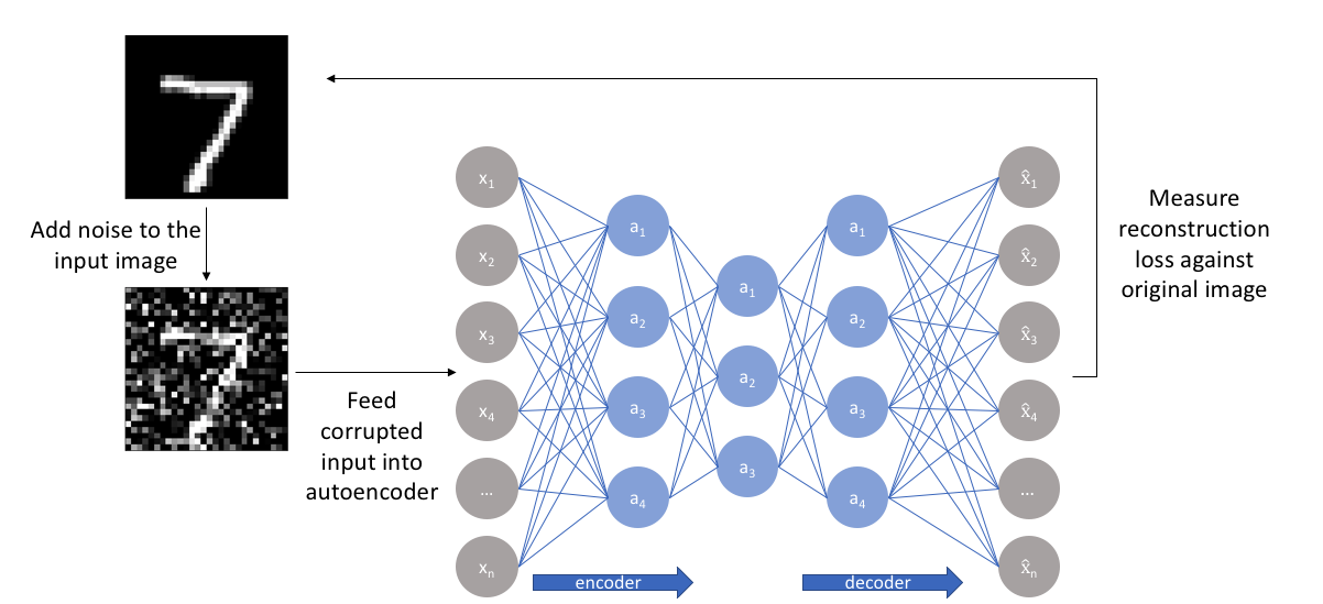
Autoencoders have been considered neural networks with identical inputs and outputs. The main goal is reproducing the input as accurately as possible while avoiding information bottlenecks. However, another way to design an autoencoder is to slightly perturb the input data but keep the pure data as the target output. With this approach, the model cannot simply create a mapping from input data to output data because they are no longer similar. So using this regularization option introduces some noise into the input while the autoencoder is expected to reconstruct a clean version of the input.

3. Contractive Autoencoders
While in the previous case, the emphasis was on making the encoder more resilient to some input perturbations, in these types of architectures, the emphasis is on making the feature extraction less sensitive to small perturbations. It is written. This is achieved by having the encoder ignore changes in the input that are not significant for reconstruction by the decoder. The main idea behind this regularization technique is that potential representations that are not important for reconstruction are reduced by the regularization factor. In contrast, important variations remain because they have a large impact on the reconstruction error is.

Figure 4 – Schematic representation of a Contractive Autoencoder
Applications of Autoencoders
If you’ve read this far, you should have the theoretical background you need to know about autoencoders. You must be wondering where the application of these structures lies in machine learning. This section sheds light on the applications of these structures.
- Dimensionality reduction was one of the first applications of representation learning. Reducing dimensions can help improve the model performance in several cases.
- Another task that benefits even more than dimensionality reduction is information retrieval.
- Other applications of autoencoders include anomaly detection, image processing, data denoising, drug discovery, popularity prediction, and machine translation.
Conclusion
That’s why I talked about autoencoders in today’s blog. Autoencoders are architectures originally designed to help with dimensionality reduction. However, its applications have multiplied many times over time. First, we briefly introduced the structure of an autoencoder and how data compression is achieved at the code layer. We then discussed different types of autoencoders and how each one helps to deal with bias-variance tradeoffs. Finally, we have finished discussing the scenarios in which autoencoders are applied in today’s world. So the key takeaways from this article are:
- The general architectural approach towards autoencoders
- The bias-variance tradeoff faced by the autoencoders
- How applying different regularization techniques can enable us to handle the tradeoff. This would enable you to think of more such algorithms and develop newer architectures.
- The areas where this type of architecture finds applicability.
I believe I could leave you with a deep theoretical understanding of the architecture and use cases of Autoencoders from this discussion in the blog. If this article excites you, I urge you to go ahead and develop one such architecture for yourself. It’s a good project to have with you.
The media shown in this article is not owned by Analytics Vidhya and is used at the Author’s discretion


