Importance of Skewness, Kurtosis, Co-efficient of Variation
This article was published as a part of the Data Science Blogathon.
Introduction
Why is a clearer understanding of skewness, kurtosis, and coefficient of variation needed for better decision-making based on their significance in a specific domain? Within what range of skewness and kurtosis a distribution shall be considered normal before selecting appropriate Statistical Tests (Hypothesis Testing)? Where does the Coefficient of variation help?
Advertently, such questions keep popping up while we work on data to perform Descriptive Analysis or apply Statistical tests to our dataset.
Be it any type of dataset expressing the status of industries/segments, when it comes to conducting Exploratory Data Analysis; our intent holds a tight grip on descriptive statistics where apart from the measure of central tendency, skewness and kurtosis also reveals some vital facts about the data given for analysis.
Even while checking the normalities assumption before conducting Statistical Tests, within what range of skewness and kurtosis a distribution shall be considered normal, understanding a range of these statistical terms remains helpful to ensure our assumption is true.
Let’s Try to understand each term, its types, significance, and application one by one.
Skewness: Definition, Types, Rang, and Examples
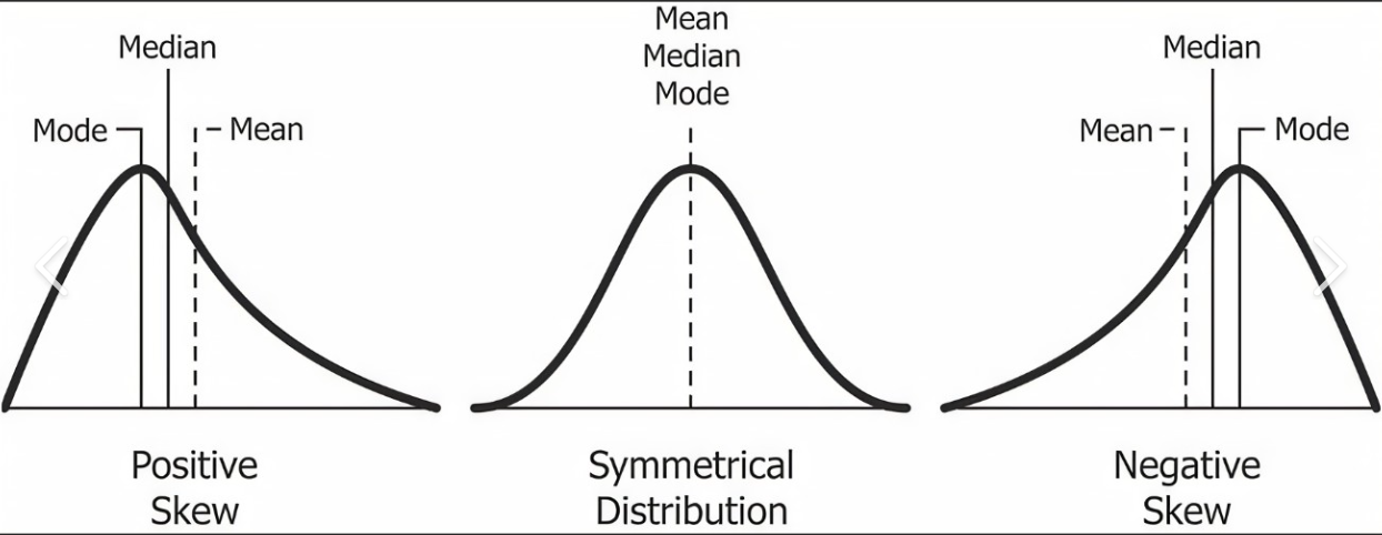
Statistical terms which express the abnormality /asymmetricity of distribution around the mean can be defined as Skewness. The presence of extreme lower or higher values (outliers) in datasets plays a vital role in pulling the distributions on either side. Mainly lower extreme values pull the distributions towards the right-hand side (median > Mean), and the entire distribution looks skewed negatively; likewise, higher extreme values pull the distribution towards the left side (mean>median), forming positive skewness. However, these data pulls act horizontally toward the left or right of the mean value.
Mean < Median: Negative or left-skewed distribution (-ve skewness)
Mean = Median: Symmetrical Distribution (Zero Skewness)
Mean > Median : Positive or Right-skewed distribution (+ ve Skewness)
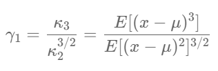
The mathematical Formula of Skewness is;
Taking an example of 1 D Dataframe, let’s try to understand skewness by looking at the data distribution and mean-median comparison. Prima facia looks a little positively skewed. But how to interpret it correctly becomes a big question. Is there any range to compare skewness? Can we consider the below distribution as approximately normally distributed?
Importing useful python library:
import pandas as pd
import numby as np
import matplotlib.pyplot as plt
import scipy.stats as st
data = np.loadtxt("dataset.txt")
plt.hist(data, bins=50);
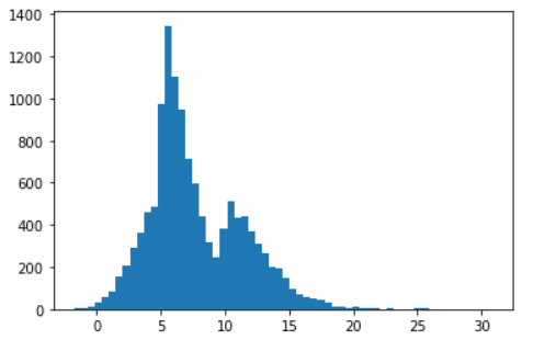
mean = np.mean(data)
print(mean)

median = np.median(data)
print(median)

In our case, the mean (7.68) is greater than the median (6.73), which means we can state that the given distribution forms a positively skewed distribution. But how much skewed is this, or shall it be considered approximately skew-normal or approximately normal? Here, Skewness Range comes to the rescue of us.
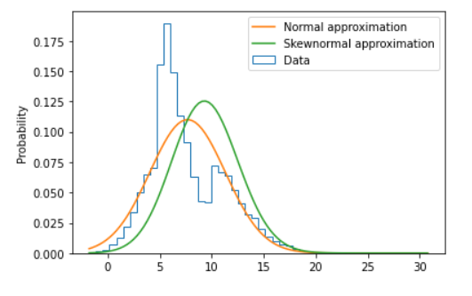
The below plot shows the difference between normal approximation and skew-normal approximation if just for ref. Finding the skewness and comparing it with its range will help to conclude it further.
Python Code to plot the distributions a pasted below:
xs = np.linspace(data.min(), data.max(), 100)

ys1 = st.norm.pdf(xs, loc=mean, scale=std)

ps = st.skewnorm.fit(data)

ys2 = st.skewnorm.pdf(xs, *ps)

plt.hist(data, bins=50, density=True, histtype="step", label="Data")

plt.plot(xs, ys1, label="Normal approximation")

plt.plot(xs, ys2, label="Skewnormal approximation")

plt.legend()

plt.ylabel("Probability");
skewness = st.skew(data)
print(skewness)
Range of Skewness
Generally, skewness values if within -0.5 to 0.5 then said distribution can be considered Normally skewed distribution and within this range, it can be also considered as approximately normally distributed.
if the skewness value varies from -0.5 to -1 for negatively skewed and 0.5 to 1 for positively skewed distribution then it indicates Moderate Skewness within the given distribution.
if the skewness value is less than -1 for Negative skewed and more than +1 for Positive skewed then said distribution is called Highly skewed accordingly.
Conclusion:
So in our case, our skewness value (0.74) falls within the range from 0.5 to 1, which means our distribution is moderately positively skewed. But cannot be considered approximately normally distributed.
Skewness Example
For positively skewed distribution, a best-suited example could be wealth distribution across the work, salary distribution in a large organization where it can be seen that higher management people (i.e. CEO / MD) get highly paid and pulls the entire distribution to the higher extreme values forms positively skewed distribution.
For negatively skewed distribution, an ideal example could be an easy exam where most students score high and fewer only get the lowest marks. Hence the presence of these failed or low-scored student pull the data towards lower extreme values and form a negative distribution.
Kurtosis, Types, Range, and Application
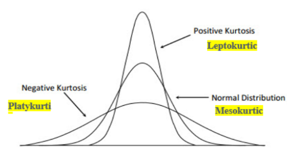
Kurtosis is a statistical measure of the peakedness of the curve for the given distribution. It defines how sharply the curve rises approaching the center of the distribution. Kurtosis also measures the presence of outliers being heavily tailed data in the case of Platykurtic. However, unlike the skewness, the data pull is acting upward or downward.
Types of Kurtosis:
If Kurtosis > 3, it is called Leptokurtic (short-tailed) with Low Standard Deviation and more data concentration near the mean and form positive kurtosis.
If Kurtosis < 3, it is called Platykurtic (long Tailed) with High Standard Deviation and shows the presence of outliers and forms negative kurtosis.
If Kurtosis = 3, then it is called Mesokurtic (like Normal distribution can be called Mesokurtic) forms zero kurtoses.
The below Figure is Just for Ref.
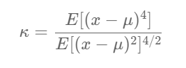
Mathematical Formula for Kurtosis (no worries, code is damme easy);
Let’s try to find out the kurtosis value of our dataset.
kurtosis = st.kurtosis(data, fisher=False)
print(kurtosis)
Range of Kurtosis
Kurtosis value can reach from 1 to + infinity. But generally, a kurtosis value = 3 (Mesokurtic) indicates a normal distribution. Kurtosis value > 3 indicates positive kurtosis (Laptokurtic) with low SD and Kurtosis value <3 indicates negative kurtosis (Platicurtic).
Range of Excess Kurtosis:
Formula; Excess Kurtosis = Kurtosis -3
In the cases of normally distributed data, excess kurtosis is taken into consideration, whose value is considered to be Zero (Excess Kurtosis = 3 -3 = 0, as per the above formula considering kurtosis =3 for normally distributed data), the minimal possible value of Excess kurtosis is -2 and ranges to infinity.
Conclusion :
In our case, as data is not normally distributed so derived value of kurtosis (3.55) can be called positive kurtosis forming Laptokurtic Type.
Skewness & Kurtosis Example
Let’s understand the importance of Kurtosis by considering a different example in investment banking.
Comparing two Investment schemes performing simultaneously, which would be better to invest with low risk?
| Data | Scheme-1 | Scheme-2 |
| Mean | 7.49 | 8.91 |
| Median | 8.5 | 9.3 |
| Mode | 8.3 | 11.9 |
| Minimum | -15.0 | -12.0 |
| Maximum | 22.0 | 16.0 |
| Range | 37 | 28 |
| Variance | 31.09 | 24.8 |
| Standard Deviation | 5.82 | 4.91 |
| Coeff. of Variation | 77.7% | 55.10% |
| Skewness | -0.63 | -1.62 |
| Kurtosis | 0.669 | 3.02 |
| Count | 499 | 499 |
| Standard Error | 0.26 | 0.21 |
Comparing here the kurtosis of both the schemes, we find scheme-2 has been performing at positive kurtosis (3.02), showing more peaked (high rise in values) than scheme-1 kurtosis value (0.669), which means in any given case, scheme-2 will give a better return. For skewness, however, both schemes seem negatively skewed (means more movement towards higher values) in which scheme-2 looks highly negatively skewed (-1.62) than scheme-1(0.63); hence the majority of values are on the higher side in scheme-2. In this case, Negative skewness is a good indicator of profit and gives positive results.
Hence comparing Skewness and Kurtosis, we can compare the performance of the two investment schemes effectively.
More Examples:
To measure Accuracy and peak performance of equipment within a certain standard deviation! In the case of manufacturing precision equipment ( aviation industries, automobile engine components, medical-surgical equipment, etc.) with the closest tolerance and lowest standard deviation.
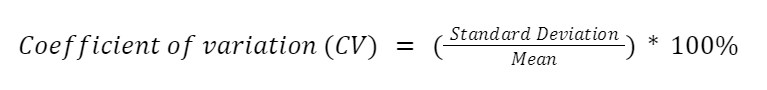
Co-efficient of Variation
It can be defined as percentage variation equal to standard deviation divided by the mean. It is a relative measure of percentage variation from the mean when variation is measured among data having different units.
In the above cases, while comparing two investment schemes, the variation coefficient shows a higher percentage variation in scheme-1 (77.7%) than in scheme-2 (55.1%). Hence, scheme-2 has a low percentage variation, so the expected risk will be low in scheme-2.
Other Applications of Co-efficient of Variations:
Comparing percentage variation within two different units of data (i.e., weight and height, Mass & Strenght, Domain of physics to dealing with Forces and their impact, etc. )
Conclusion
Statistical measures of variation help to make better decisions if their values are interpreted and understood well. The above examples show how crucial such variations are in real-work scenarios.
- Skewness measures horizontal pulls of data on either side of the mean (either positive or negative) basis on the presence of extreme values (lower or extreme). Its relevance/significance is contextural based on the domain/segment.
- Kurtosis expresses the vertical upward or downward pull of data-based data distribution near the mean and its relative standard deviation. This also indicates the presence of outliers based on the type of either-sided tails (flatter, heavier).
- Co-efficient variation measures the percentage (%) variation, so when comparing two features having different units, then % variation helps for better clearing.
I hope you liked my article on skewness, kurtosis, and co-efficient of variance in data science. Connect me at [email protected] for more information!
https://www.linkedin.com/in/shailesh-shukla-264b3222
The media shown in this article is not owned by Analytics Vidhya and is used at the Author’s discretion.


