Step-by-Step Working of Decision Tree Algorithm

Rakesh Kanth 14 Feb, 2023 • 8 min read

Introduction

I hope by now you are familiar with linear and logistic regression. In those algorithms, the major disadvantage is that it has to be linear, and the data needs to follow some assumption. For example, 1. Homoscedasticity 2. multicollinearity 3. No auto-correlation and so on. But, In the Decision tree, we don‘t need to follow any assumption. And it also handles non-linear data. Now, let’s understand what a decision tree is. It is a supervised machine-learning algorithm. It can handle both classification and regression.

Decision Tree Analysis is a generic predictive modeling tool with applications in various fields. Decision trees are generally built using an algorithmic approach that identifies multiple ways to segment a data set based on certain factors. It is one of the most extensively used and practical supervised learning algorithms. Decision Trees are a non-parametric supervised learning method that can be used for classification and regression applications. The goal is to build a model that predicts the value of a target variable using basic decision rules derived from data attributes.

The decision rules are typically written in the form of if-then-else expressions. The deeper the tree, the more complicated the rules and the more accurate the model.

Learning Objective

This blog explores why decision trees are easy to interpret with their structure. We will see plenty of examples to understand the flow of the decision tree algorithm. Through hands-on demonstrations, we will also understand how to split the nodes of a decision tree. And we will finally implement it via python using a popular dataset.

This article was published as a part of the Data Science Blogathon.

How can we create a simple decision tree?
A Decision Tree splits the nodes in a decision tree in two ways.
Splitting the nodes in the Decision Tree
Gini Impurity: How to understand it by hand?
Taking a deeper look at the idea of Entropy and Information gain
5.1 Step1 : Entropy
5.2 Step2: Information gain
Conclusion

How Can We Create A Simple Decision Tree?

Decision trees are one of the most popular and accessible algorithms out there. It is very intuitive because it works exactly the way we think. For example, to decide about our career options or to buy a product or house. In simple lines, the daily decisions are identical to the decision tree model.

So, how was the structure built? And why it’s similar to the way we think. Let’s understand with an example below.

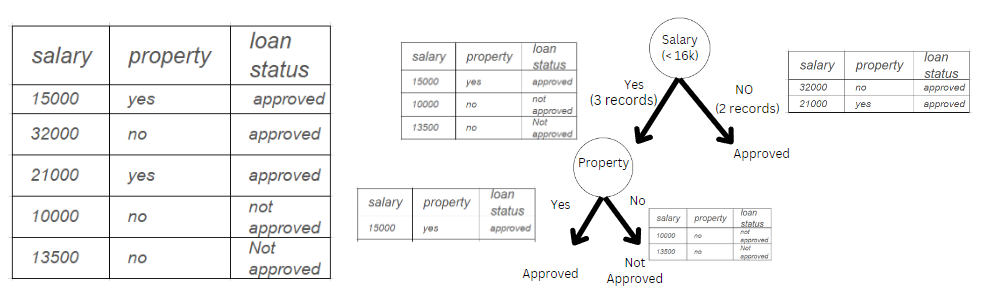
Image 1

In the above example, we are trying to understand whether a person gets a loan based on salary and property. We can consider Y variable (loan approval) column. There are two input parameters: the X1 variable – salary(in rupees) and the X2 variable – property(land or house). We have built a small decision tree.

Condition 1: If the salary is less than Rs. 16000, we need to check whether they have property. If yes, give them the loan.

Condition 2: Give them a loan if the salary is more than Rs. 16000.

The example above is very straightforward to understand the structure. But before moving forward, we need to understand a few important questions.

Question 1-> What are terminologies used in a decision tree? We will understand with an example below.

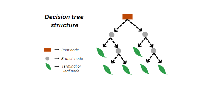
Image 2

Question 2 -> Why did we select the salary column first instead of the property column in Image 1? We considered the salary column as an example of building a tree. But, when we are working on the real-world dataset, we cannot choose the column randomly. Read the following section to know what process we use in real-time.

Splitting the Nodes in a Decision Tree

Now, Let’s consider the dataset below in Image 3 for a detailed understanding. Again we need to answer the question before building the decision tree model.

Which column must be selected as the root node in the dataset below?

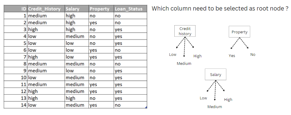
Image 3

To answer the above question, we need to check how good each column is and What qualities it has to be a root node. To know which column we will be using:

Gini
Entropy and Information Gain

Let’s understand one by one with hands-on examples.

Gini Impurity in Decision Tree: How to Understand It?

First, We will calculate the Gini impurity for column 1 credit history. Likewise, we must calculate the Gini impurity for the other columns like salary and property. The value we will get is how impure an attribute is. So, the lesser the value lesser the impurity the value ranges between(0-1).

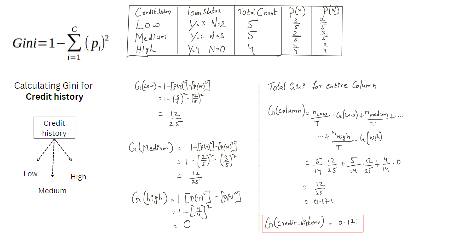
Image 4

In the above image4, we got Gini for each class in credit history.

G(Low) = 12/25

G(medium) = 12/25

G(High) = 0

Then we calculated the Total Gini for the entire credit history column. Let’s understand the formula.

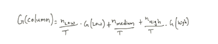
Image 5

n = Total count of that class in the column credit history

T = Total count of instances. In our case, it is 14( we have a total of 14 rows in the Image3)

Example: nlow/T can be written as 5/14. Here we got 5 from the count of Credit_history(low) we see in Image 4 (3rd column).

Image 6

Finally, We got the Impurity for the column Credit history = 0.171.

Now, We have to calculate the Gini for each Feature as we did for the credit_history feature above.

After calculating Gini for both features,

We will get Impurity for the column Salary = 0.440 and Property = 0.428. For a detailed understanding, we can check the image below.

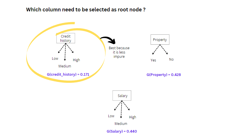
Image 7

Similarly, we continue the process of selecting the branch node, and we can build a Decision Tree. We will now try a different method for carrying out the same process of building a decision tree below.

The Idea of Entropy and Information Gain

Entropy is also a measure of randomness or impurity. It is helpful while splitting the nodes further and making the right decision. The formula for entropy is:

Image 8

But with entropy, we will also be using Information gain. So, Information gain helps to understand how much information we get from each feature.

Image 9

But Before going further, we need to understand why we need entropy and information gain and why we need to use them. Let’s consider the example we have used in Gini. In that, we have a Credit history, Salary, and property. Again we have to start from the beginning. What do I mean by beginning from scratch? We must start calculating Entropy and information gained from each attribute and select a root node. That means we have 2 popular ways of solving the problem 1. Gini, 2. Entropy and information gain. We have already learned how to build a decision tree using Gini. From here on, we will understand how to build a decision tree using the Entropy and information gain step by step.

Before calculating the entropy for input attributes, we need to calculate the entropy for the target or output variable. In our dataset, the output variable is loan status.

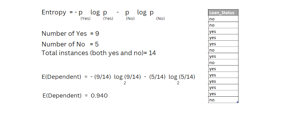
Image 10

Select the attribute out of 3 attributes as a root node in the data set we have seen in image 3. We need to calculate Information gain for all the 3 independent attributes.

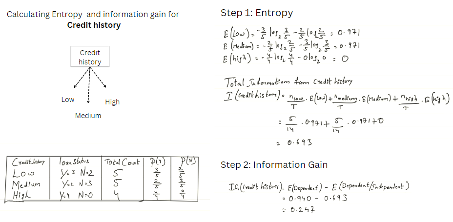
Image 11

In the above image 11, we have calculated Entropy for the column Credit history. We can divide the calculations into two steps to understand the math above.

Step1: Entropy

We have calculated the entropy for each class in the credit _history column.

We got,

E(Low) = 0.971
E(Medium) = 0.971
E(High) = 0

Then calculate the total information for the whole column Credit history.

At the end of step 1, we have done the same math as we have done in the Gini Impurity section above. We can refer to image 5 for a better understanding. Then we got a value.

I(Credit History) = 0.693

Step 2: Information Gain

This is the easiest step; we must subtract the I(independent) from E(Dependent). You can find the formula in images 9 and image 10.

IG(Credit History) = 0.247

We have to calculate the Entropy and information Gain for the remaining features as we did for the credit history feature above in image 11.

After repeating the same process for the other feature, we will get

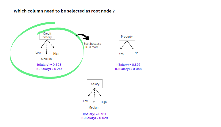
Image 12

The above image shows that credit history is the best attribute as a root node because the Information gain is more.

Similarly, we continue the process of selecting the branch node, and we can build a complete decision tree.

Which method is best, Gini Or Entropy with information Gain?

We cannot say which is best; we have to try both and see. Which one fits our data well because both have their advantages and disadvantages?

Python Implementation

from sklearn import datasets
data = datasets.load_breast_cancer()
X = data.data
y = data.target

In the above code, we are importing the popular inbuilt dataset from sklearn (breast cancer dataset), and we have used variable X for the Input data and Y for the target data.

from sklearn.model_selection import train_test_split
X_train, X_test, y_train, y_test = train_test_split(X,y, test_size=0.2, random_state=0)

We must divide the data into training(80%) and testing(20%).

from sklearn.tree import DecisionTreeClassifier
model = DecisionTreeClassifier(criterion='gini')
model.fit(X_train, y_train)

With the above code, we are trying to build the decision tree model using “Gini.” we can also change the criterion = “entropy.”

expected = y_test
predicted = model.predict(X_test)

In the above code expected variable has actual values. The predicted variable has the predicted values by the decision tree.

from sklearn import metrics
print(metrics.confusion_matrix(expected, predicted))

The confusion matrix helps us to decide how well a model performs using precision, recall, and F1 scores.

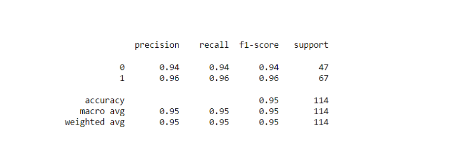
Image 13

Conclusion

In this article, we started with the introduction, explaining the difference between the linear and the decision tree models. Next, we understood the terminologies used in the decision trees and how a node will be split using Gini, entropy, and information gain. We also understood the complete math(hands-on) behind all of them. Finally, We used python for implementation.

Key Takeaways:

1. Decision trees are easy to interpret. With their structure, we can understand what will be the possible outcome.

2. By learning this, we handle both regression and classification problems

3. In the article, we have learned about Gini and entropy, and we can even make the feature selection.

4. Unlike linear and logistic regression, the Decision tree is a non-parametric algorithm which means it doesn’t need any assumption to build the model.

Did you enjoy my article? Share with me in the comments below.

Get insights on Decision Tree Algorithm for Classification by reading the below blog: