Unveiling Power of Filters in Medical X-ray Image Processing
Introduction
“Image processing” may seem new to you. Still, we all do image processing in our daily life, like blurring, cropping, de-noising, and also adding different filters to enhance an image before uploading it to social media. Sometimes it is the app that you use has that task automated (i.e., deep learning), so you can use the enhanced image right after the shot. Like, processing the raw medical image is also a very crucial step in any automated medical diagnostics e.g. classification of different kinds of tumors, pneumonia from a chest x-ray, brain strokes from a CT-Scan, internal hemorrhage from MRI, etc.
In this article, we will discuss different types of filters used in image processing, especially chest X-Ray, for extracting important areas from the images.
Learning Objectives
- Multidimensional image processing technique.
- Application of Laplace-Gaussian, Gaussian-Gradient-Magnitude edge detection operator on Chest X-ray images.
- The working of Sobel and Canny filter and its application.
- Use of Numpy for masking an image to separate important segments.
- Use of Matplotlib library to plot multiple images together.
This article was published as a part of the Data Science Blogathon.
Table of Contents
- Dataset
- Setup Project Environment
- Examine X-ray Images
- Edge Detection on the X-ray Image
- How to apply masks to X-ray images for extracting important features from the raw images?
- Conclusion
Dataset
The dataset we use in this article is from Kaggle Pneumonia X-ray Image.
Download Link
Chest X-Ray pneumonia image.
Data Description
- Total number of observations (images): 5,856
- Training observations: 4,192 (1,082 normal cases, 3,110 lung opacity cases)
- Validation observations: 1,040 (267 normal cases, 773 lung opacity cases)
- Testing observations: 624 (234 normal cases, 390 lung opacity cases)
- Setup Project Environment
We use anaconda for project development. To create a new project environment, follow the below instruction.
1. Open your terminal and type these
$ conda create --name imgproc python=3.9

$ conda activate imgproc
2. Now, Install the necessary libraries
pip install numpy matplotlib scipy imageioExamine X-ray Images
I downloaded and extracted the zip file in the “image” folder. You can see the image data is in JPEG format.
To read the image file, we use the ImageIO library. The medical industry mainly works with DICOM format, and although “imageio” can read DICOM format, we will only work with JPEG format today.
Create a list of all the image files in the train normal folder.
import os
import glob

# Supported image file extensions
image_extensions = ['*.jpg', '*.jpeg', '*.png']

image_list = []

for ext in image_extensions:
    image_files = glob.glob(os.path.join(image_dir, ext))
    image_list.extend(image_files)

print("LIst of image files in Train/normal")
for image_path in image_list:

    print(image_path)
Load a single image
import os
import imageio.v3

FILE_PATH = "./images/x-rays/pneumonia-xray/train/normal/"

original_img = imageio.v3.imread(os.path.join(FILE_PATH, "IM-0115-0001.jpeg"))
Now see the shape and data type of the image
print(f"Shape of the image: ", original_img.shape)
print(f"Data Type of the image: ", original_img.dtype)
And the chest X-ray image
import matplotlib.pyplot as plt

plt.imshow(original_img, cmap="gray")
plt.axis("off")
plt.show()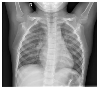
Create a GIF file to see the first 10 images from the train folder.
First, create a list of 10 images:
import numpy as np
num_img = 10
arr = []

for i, img in enumerate(image_list):
    if(i == num_img):
        break
    else:
        temp_img = imageio.v3.imread(f"{img}")
        arr.append(temp_img)
Creating GIF:
GIF_PATH = os.path.join("./images/","x-ray_img.gif")
imageio.mimwrite(GIF_PATH, arr, format=".gif", fps=1)
The gif file is not added here, because the editor renders it.
Now, dive deep into edge detection.
Edge Detection on the X-ray Image in Image Processing
What is Edge Detection?
It is a mathematical operation applied to the directional changes in color or image gradient. It is used for detecting the boundary of an image. There are many operators for detecting edges e.g., gradient technique, Sobel operator, Canny edge detection, etc. See below examples
Original Image
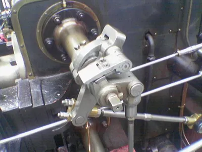
Source: Wikipedia Sobel Operator
Detected Edge of the Valve
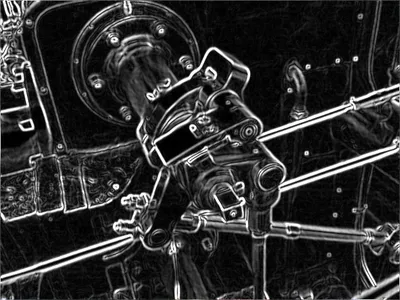
Source: Wikipedia Sobel Operator
Types of Edge Detection Algorithms
Now we apply different types of edge detection algorithms to our Chest x-ray images. Let’s get this started!
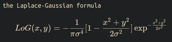
1. The Laplace-Gaussian Filter
In this method, the Laplacian method focuses on changing the pixel intensity, and the Gaussian method is used to remove noise from the images.
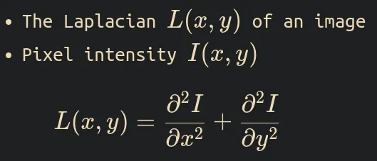
What is Laplacian function of the image?
The Laplacian of the image is defined as the divergence of the gradient of the pixel intensity function, which is equal to the sum of the I(x,y) function’s second spatial derivatives in cartesian coordinates.
If The Laplacian is L(x,y) and the pixel intensity function I(x,y). The formula is
What is Gaussian?
The Gaussian or normal distribution function is a probability distribution used in statistics. Its shape is like a bell. That’s why sometimes it’s called the bell shape curve. It is significant that the curve is symmetric around the mean.
Formula:
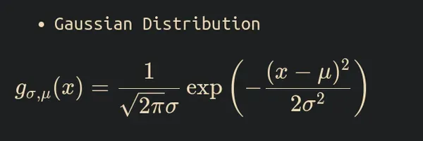
Here, the Greek symbols sigma and mu are the standard deviation and mean of the distribution, respectively. Below is an example plot.
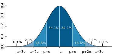
Source: Wikipedia
In image processing, Normal distribution is used to reduce noise from the image. We can smoothen the image by applying a Gaussian filter an image and reducing the noise.
The Gaussian filter process is a convolutional operation that replaces each pixel value of the image by taking the weighted average of the neighboring pixel values. e.g., the blurred image below is produced after applying the Gaussian Filter on the top image.

Source: Wikipedia
And you might wonder why it is called the Gaussian. The answer is to take the weighted average of the neighboring pixels of the image. The Gaussian distribution determines the weight.
The formula of the 2nd derivative of Gaussian distribution is
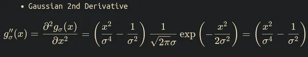
The Laplace-Gaussian operator formula is
Enough math is done now implementation.
Implementation
We implement the Laplace Gaussian operation on an X-ray image using SciPy ndimage’s gaussina_laplace() function with a standard deviation of 1.
from scipy import ndimage

xray_LG = ndimage.gaussian_laplace(
    original_img,
    sigma=1
)
Now, we compare both the original and filtered images side by side. So, first, we create a function to plot the images using the Matplolib pyplot library.
def plot_xray(image1, image2, title1="Original", title2="Image2"):
    fig, axes = plt.subplots(nrows=1, ncols=2, figsize=(10, 10))

    axes[0].set_title(title1)
    axes[0].imshow(image1, cmap="gray")
    axes[1].set_title(title2)
    axes[1].imshow(image2, cmap="gray")
    for i in axes:
        i.axis("off")
    plt.show()
This function will create the plot of both images.
Now see the results.
plot_xray(original_img,xray_LG, title2="Laplace gaussian edges")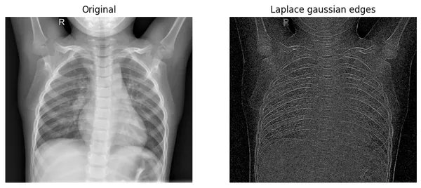
The operator especially focuses on where the pixel intensity is changed very rapidly. If you look at the original image’s bones, you find that there are pixels in rapid change. Our edges of the filtered image are exactly showing those changes.
Now proceed to the next filter.
2. Gaussian Gradient Magnitude
What is Gaussian gradient magnitude?
We already know what Gaussian or normal distribution in the Laplace-Gaussian filter is. Now, the Gradient of an image is the changes in the intensity or color to a certain direction.
Image gradient example.
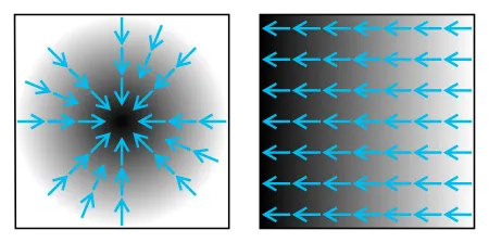
Mathematically, first, the algorithm applies the Gaussian filter on the image in both the x-axis and y-axis or horizontally and vertically. It blurs the image, but the overall structure of the image is intact.
Second, The magnitude is calculated by taking both gradient directions’ square root or Euclidean distance.
In this method of edge detection, we remove the high-frequency components from the image using multidimensional gradient magnitude with Gaussian derivative.
In image processing, high-frequency means the edge part, and low-frequency means the body part of that image.
Implementation
We use Scipy ndimage’s gaussian_gradient_magnitude() with a standard deviation(sigma) of 2.
xray_GM = ndimage.gaussian_gradient_magnitude(
    original_img,
    sigma=2
)
Now, see the result by plotting
plot_xray(original_img, xray_GM, title2="Gaussian Gradient Mag")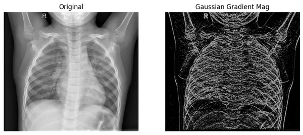
Here, we can see that the filtered image extracts the edges from the original image, where color values change rapidly. And in comparison with the Laplace-Gaussian method, it shows edges better.
3. Sobel Filter
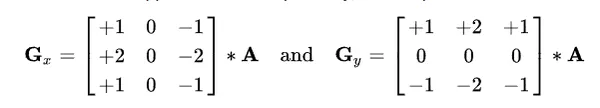
The Sobel filter, also known as the Soble-Feldman operator used in image processing. It uses convolution operation on the image to calculate the approximation of the gradient.
How does it work?
There are two separate [3 by 3] kernels for each direction. One for the x-axis or horizontal and one for the y-axis or vertical. These kernels convolve on the original image to calculate the gradient approximation of the original image in both horizontal and vertical directions.
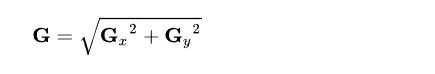
Then, It will calculate the magnitude by taking the square root of both directional gradients.
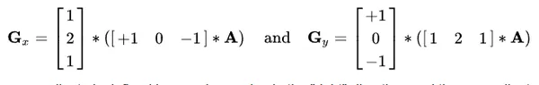
If A is an image and G_x and G_y are horizontal and vertical derivative approximations at each point.
The computation will be like
Compute the gradient with smoothi
Calculating the magnitude of both gradients.
Now, using all the information, we can calculate the gradient direction using

For example, the direction angle big theta will be 0 for the vertical edge.
Implementation
a. To implement the Sobel filter, we use ndimage’s sobel() function. We must apply the Sobel filter on the x-axis and y-axis of the original image separately.
x_sb = ndimage.sobel(original_img, axis=0)
y_sb = ndimage.sobel(original_img, axis=1)
b. Then, we use np.hypot() to calculate euclidean distance of sobel_x and sobel_y
c. Last, normalize the image.
# taking magnitude
sobel_img = np.hypot(x_sb, y_sb)

# Normalization
sobel_img *= 255.0 / np.max(sobel_img)
Now, the image becomes float16 format, so we must transform it into float32 format for better compatibility with the matplotlib.
print("The data type - before: ", sobel_img.dtype)

sobel_img = sobel_img.astype("float32")

print("The data type - before: ", sobel_img.dtype)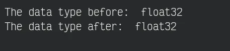
Let’s see the results
We will plot the original image along with both grayscale and CMRmap colormap scale for better visualization of filtered images.
fig, axes = plt.subplots(nrows=1, ncols=3, figsize=(15, 15))

axes[0].set_title("Original")
axes[0].imshow(original_img, cmap="gray")
axes[1].set_title("Sobel_edges: grayscale")
axes[1].imshow(sobel_img, cmap="gray")
axes[2].set_title("Sobel_edges: CMRmap")
axes[2].imshow(sobel_img, cmap="CMRmap")
for i in axes:
    i.axis("off")
plt.show()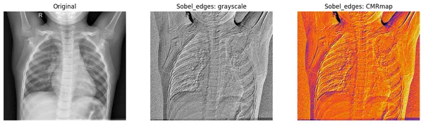
In the resulting plot, the Sobel filter focuses more on the lung area of the chest X-ray.
4. The Canny Filter
According to Wikipedia, The canny filter or canny edge detection is a technique that applies multiple algorithms to the images to get the results. It is developed by John.F.Canny in 1986.
In general, the algorithm works as
a. Noise Reduction
It uses the Gaussian filter (deep learning) to reduce noise from the images. Here, it uses the 5 by 5 Gaussian kernel for convolution.
b. Calculate Intensity Gradient
We already know how to find the intensity gradient in the Sobel filter section. In short, It applies the Sobel filter on the smoothened image in the horizontal and vertical direction. After that, it calculates the gradient magnitude and gradient direction.
c. Non-maximum Suppression
It is a deep learning technique to remove the pixel which does not constitute the edge.
d. Hysteresis Thresholding
In this phase, the deep learning algorithm calculates the edges and those not. There are two threshold values, min_val and max_val, for the edges. If the certain edge is more than max_val, then it is considered a sure edge, and if the edge is below the min_val, then it is considered sure not edge, so it will be discarded.
The choice of min_val and max_val is important for getting correct results.
Implementation
To get the canny image,
first, apply the Fourier Gaussian filter on the original image to get a smoother image.
fourier_gau = ndimage.fourier_gaussian(
    original_img,
    sigma=0.05
)
Second, we calculate both the directional gradient using Prewitt from Scipy ndimage.
x_prewitt = ndimage.prewitt(fourier_gau, axis=0)
y_prewitt = ndimage.prewitt(fourier_gau, axis=1)
And the last, We calculate the gradient by taking the square root of both gradients. And then normalizing the image.
xray_canny = np.hypot(x_prewitt, y_prewitt)
xray_canny *= 255.0 / np.max(xray_canny)
The data type of the resulting image
print(f"the data type - {xray_canny.dtype}")Let’s see the results
fig, axes = plt.subplots(nrows=1, ncols=4, figsize=(20, 15))

axes[0].set_title("Original")
axes[0].imshow(original_img, cmap="gray")
axes[1].set_title("Canny edge: prism")
axes[1].imshow(xray_canny, cmap="prism")
axes[2].set_title("Canny edge: nipy_spectral")
axes[2].imshow(xray_canny, cmap="nipy_spectral")
axes[3].set_title("Canny edges: terrain")
axes[3].imshow(xray_canny, cmap="terrain")
for i in axes:
    i.axis("off")
plt.show()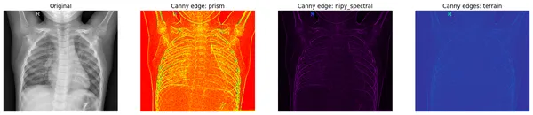
How to Apply Masks to X-ray Images for Extracting Features-Based Image Processing from the Raw Images?
By masking certain pixels of an image, we can extract the features from the original images.
let’s show some images first.
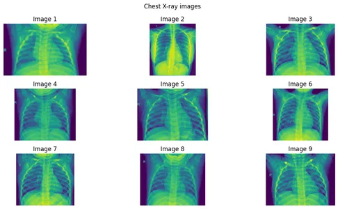
Step 1: Create an image array of 9 images.
images = [
    imageio.v3.imread(image_list[i]) for i in range(9)
]
Step 2: Plotting the Images
n_images = len(images)
n_rows = 3
n_cols = (n_images + 1) // n_rows
fig, axes = plt.subplots(n_rows, n_cols, figsize=(12, 6))
axes = axes.flatten()
for i in range(n_images):
if i < n_images:
axes[i].imshow(images[i])
axes[i].axis('off')
axes[i].set_title(f"Image {i+1}")
else:
axes[i].axis("off")
for i in range(n_images, n_rows * n_cols):
axes[i].axis("off")
fig.suptitle("Chest X-ray images")
plt.tight_layout()
plt.show()

Now, See some basic statistics of pixel values
print("The data type of the X-ray image is: ", original_img.dtype)
print("The minimum pixel value is: ", np.min(original_img))
print("The maximum pixel value is: ", np.max(original_img))
print("The average pixel value is: ", np.mean(original_img))
print("The median pixel value is: ", np.median(original_img))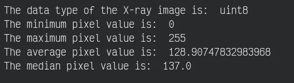
Step 3: Plotting the Pixel density distribution of all the above images.
fig, axes = plt.subplots(n_rows, n_cols, figsize=(12, 6))
axes = axes.flatten()

for i in range(n_images):
    if i < n_images:

        pixel_int_dist = ndimage.histogram(images[i],
            min=np.min(images[i]),
            max=np.max(images[i]),
            bins=256)
        axes[i].plot(pixel_int_dist)
        axes[i].set_xlim(0, 255)
        axes[i].set_ylim(0, np.max(pixel_int_dist))
        axes[i].set_title(f"PDD of img_{i+1}")


fig.suptitle("Pixel density distribution of Chest X-ray images")
plt.tight_layout()
plt.show()
Step 4: Extracting features from images using masking
We use np.where() with the threshold value of 150. This means the pixel greater than 150 will stay otherwise will become 0.
fig, axes = plt.subplots(n_rows, n_cols, figsize=(12, 6))
axes = axes.flatten()

for i in range(n_images):
    if i < n_images:
        noisy_image = np.where(images[i] >150, images[i], 0 )
        axes[i].imshow(noisy_image, cmap="gray")
        axes[i].set_title(f"Image {i+1}")
    else:
        axes[i].axis("off")

for i in range(n_images, n_rows * n_cols):
    axes[i].axis("off")

fig.suptitle("Chest X-ray images")
plt.tight_layout()
plt.show()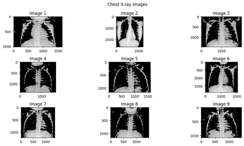
Now, we can see that the masked pixel is not showing or blackened by np.where() method.
Conclusion
Edge detection is a very important task for healthcare industries, deep learning image classification projects, and Object detection projects. In this article, we learn lots of techniques today. You can apply these techniques in any image classification project on Kaggle competitions. And also you can further study the subject to come up with better techniques.
Key takeaways
- Learning about image processing in deep learning.
- How modern mathematics is used in Image processing of deep learning.
- Laplacian gradient and application of Gaussian distribution on image processing.
- Sobel and canny filter operation.
- Application of masking technique for features extraction in deep learning.
All the codes of this article are available here (look for the x-ray-process.ipynb file)
Thank you for reading, If you like the article please like and share it with your fellow learners. Follow me on LinkedIn
The media shown in this article is not owned by Analytics Vidhya and is used at the Author’s discretion.


