Object Localization with CNN-based Localizers

Introduction

Object Localization refers to the task of precisely identifying and localizing objects of interest within an image. It plays a crucial role in computer vision applications, enabling tasks like object detection, tracking, and segmentation. In the context of CNN-based localizers, object localization involves training a convolutional neural network (CNN) to predict the coordinates of bounding boxes that tightly enclose the objects within an image.

The localization process typically follows a two-step pipeline, with a backbone CNN extracting image features and a regression head predicting the bounding box coordinates.

Learning Objectives

• To understand the basics of Convolutional Neural Networks (CNNs).
• Explain CNN architecture for localization models.
• Implement localizer architecture using a pre-trained CNN model for localization.

This article was published as a part of the Data Science Blogathon.

Convolutional Neural Networks (CNNs)

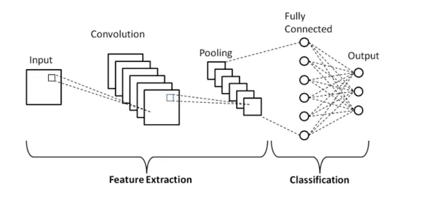
Convolutional Neural Networks (CNNs) are a class of deep learning models used for image analysis.

Their architecture consists of an input layer that takes in the image data, followed by convolutional layers that learn and extract features using convolutional filters. Activation functions introduce non-linearities while pooling layers reduce spatial dimensions. Fully connected layers at the end make final predictions.

CNNs learn hierarchical features, starting with low-level features like edges and progressing to complex and abstract features like shapes and object compositions.

During the training phase of a CNN, the network learns to recognize and extract different levels of features automatically. The initial layers capture low-level features such as edges, corners, and textures, while deeper layers learn more complex and abstract features like shapes, object parts, and object compositions. The hierarchical structure of a CNN allows it to learn representations that are increasingly invariant to variations in translation, scale, rotation, and other image transformations.

CNN-based Localizer Architecture

The CNN-based localizer model for object localization consists of 3 components:

1. CNN Backbone

Incorporating the Power of SQL: Choosing a Standard CNN Architecture (such as ResNet 18, ResNet 50, VGG, etc.) for Finetuning Pre-trained Models on Imagenet Classification Tasks. Enhancing the Backbone Network with Additional CNN Layers for Feature Map Size Reduction

2. Vectorizer

The output of the CNN backbone is a 3D tensor. But the resultant output of the Localizer is a 1D vector with four values corresponding to each coordinate for the bounding box. To convert the 3D tensor into a vector, we employ a vectorizer or utilize a Flatten layer as an alternative approach.

3. Regression Head

We construct a fully connected regression head specifically for this task. After that, the feature vector, obtained from the backbone, is fed to the regression head. The regression head consists of 4 nodes at the end corresponding to the (x1, y1, x2, y2) or any other equivalent bounding box representations.

Understanding the Model Architecture Better

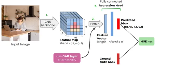
The figure shows a common CNN-based localizer model architecture. In short, the CNN backbone takes in an RGB image, then generates a feature map. We then use a flattened layer or a Global Average Pooling layer to form a 1-dimensional feature vector. The fully connected regression head takes in the feature vector and gives predictions.

The CNN network maintains a fixed size for the input image, and we employ a Flatten layer to convert the feature map acquired from the CNN backbone into a vector. However, when adaptive layers like GAP (Global Average Pooling) are utilized, there is no requirement to resize the image.

Training the Localizer

Import Necessary Libraries

import ast
import math
import os

import cv2
import pandas as pd
import numpy as np
import matplotlib.pyplot as plt
import tensorflow as tf

from functools import partial

from tensorflow.data import Dataset
from tensorflow.keras.applications import ResNet50
from tensorflow.keras import layers, losses, models, optimizers, utils 

Building the Components

The architecture takes an input image of size 300×300 with 3 color channels.

• The backbone processes the image and extracts high-level features.
• The vectorizer then computes a fixed-length vector representation of these features.
• Finally, the regression head takes this vector and performs regression, outputting a 4-dimensional vector as the final prediction.

IMG_SHAPE = (300, 300)

backbone = models.Sequential([
    ResNet50(include_top=False, 
    weights='imagenet', 
    input_shape=IMG_SHAPE + (3,)),
    layers.Conv2D(1024, 3, 2, activation='relu'),
    ], name='backbone' )

vectorizer = layers.GlobalAveragePooling2D(name='GAP_vectorizer')

regression_head = models.Sequential([
    layers.Dense(512, activation='relu'),
    layers.Dense(4)
], name='regression_head')

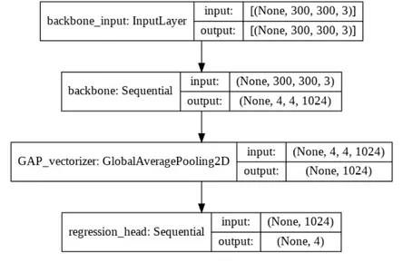
Building the Model

It defines a complete model by combining the previously defined components: the backbone, the vectorizer, and the regression head.

bbox_regressor = models.Sequential([
    backbone, 
    vectorizer,
	regression_head
])

bbox_regressor.summary()

utils.plot_model(bbox_regressor, "localizer.png", show_shapes=True)

Download the Dataset

We are using a selfies dataset. The Selfie dataset contains 46,836 selfie images. We generate bounding boxes for faces using Haar Cascades. A CSV file is available which consists of an image path and bounding box coordinates for about 22K images.

The dataset is available at:

https://www.crcv.ucf.edu/data/Selfie/Selfie-dataset.tar.gz

Generating Data Batches

DataGenerator class is responsible for loading and preprocessing existing data for the localization task.

• It takes an image directory and a CSV file with image paths and bounding box information as input.
• The class divides the data into training and testing subsets based on the provided fractions.
• During generation, the class preprocesses each image by resizing it, converting color channels, and normalizing pixel values.
• Bounding box coordinates are also normal.

The generator yields the preprocessed image and corresponding bounding box for each data sample.

class DataGenerator(object):
    def __init__(self, img_dir, _csv_path, train_max=0.8, test_min=0.9, target_shape=(300, 300)):
        for k, v in locals().items():
            if k != "self" and not k.startswith("_"):
                setattr(self, k, v)
        
        self.df = pd.read_csv(_csv_path)
        
    def __len__(self):
        return len(self.df)
        
    def generate(self, phase):
        assert phase in [None, 'train', 'test']
        _df = self.divide_data(phase)

        for rel_img_path, bbox in _df.values:
            img, bbox = self.preprocess_data(rel_img_path, bbox)
            img = tf.constant(img, dtype=tf.float32)
            bbox = tf.constant(bbox, dtype=tf.float32)
            yield img, bbox

    def preprocess_data(self, rel_img_path, bbox):
        bbox = np.array(ast.literal_eval(bbox))

        img_path = os.path.join(self.img_dir, rel_img_path)

        img = cv2.imread(img_path)
        img = cv2.cvtColor(img, cv2.COLOR_BGR2RGB)
        _h, _w, _ = img.shape
        img = cv2.resize(img, self.target_shape)
        img = img.astype(np.float32) / 127.0 - 1

        bbox = bbox / np.array([_w, _h, _w, _h])

        return img, bbox # np.expand_dims(bbox, 0)

    def divide_data(self, phase):
        train_max = int(self.train_max * len(self.df))
        
        _df = None
        
        if phase is None:
            _df = self.df
        elif phase == 'train':
            _df = self.df.iloc[:train_max, :].sample(frac=1)
        else:
            _df = self.df.iloc[train_max:, :]
            
        return _df 

Loading and Creating the Dataset

This uses the DataGenerator class to create training and testing datasets using TensorFlow’s Dataset API.

• It creates training and testing datasets using TensorFlow’s Dataset API.
• We generate the training dataset by invoking the ‘generate’ method of the DataGenerator instance, specifying the ‘train’ phase.
• Generate the testing dataset with the ‘test’ phase.
• Both datasets are shuffled and batched with a batch size of 16.

The resulting train_dataset and test_dataset are TensorFlow Dataset objects, ready for further processing or training of a model.

IMG_DIR = 'Selfie-dataset/images'
CSV_PATH = '3-lv1-8-4-selfies_dataset.csv'

BATCH_SIZE = 16

dataset_generator = DataGenerator(IMG_DIR, CSV_PATH)
train_max = int(len(dataset_generator) * 0.9)

train_dataset = Dataset.from_generator(partial(dataset_generator.generate,
 phase='train'), output_types=(tf.float32, tf.float32), 
 output_shapes = (IMG_SHAPE + (3,), (4,)))
 
train_dataset = train_dataset.shuffle(buffer_size=2 * BATCH_SIZE).batch(BATCH_SIZE)

test_dataset = Dataset.from_generator(partial(dataset_generator.generate, 
  phase='test'),output_types=(tf.float32, tf.float32), 
  output_shapes = (IMG_SHAPE + (3,), (4,)))

test_dataset = test_dataset.shuffle(buffer_size=2 * BATCH_SIZE).batch(BATCH_SIZE)

Loss Function and Performance Metric

Several loss functions for regression can be used to train a bounding box localizer. The regression loss functions like MSE, and Smooth L1 are used in a similar fashion as in the case of other regression tasks and are applied between the ground truth bounding box vector and predicted bounding box vector.

Intersection over Union (IoU) is a common performance metric used in bounding box regression.

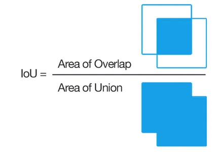
The function defines a set of functions for calculating the Intersection over Union (IoU) and evaluating the performance of a model’s predictions. It provides the means to calculate IoU, evaluate predictions in terms of loss and IoU, and assign the evaluation criterion to a variable.

def cal_IoU(b1, b2):
    zero = tf.convert_to_tensor(0., b1.dtype)

    b1_x1, b1_y1, b1_x2, b1_y2 = tf.unstack(b1, 4, axis=-1)
    b2_x1, b2_y1, b2_x2, b2_y2 = tf.unstack(b2, 4, axis=-1)
    
    b1_width = tf.maximum(zero, b1_x2 - b1_x1)
    b1_height = tf.maximum(zero, b1_y2 - b1_y1)
    b2_width = tf.maximum(zero, b2_x2 - b2_x1)
    b2_height = tf.maximum(zero, b2_y2 - b2_y1)
    
    b1_area = b1_width * b1_height
    b2_area = b2_width * b2_height

    intersect_x1 = tf.maximum(b1_x1, b2_x1)
    intersect_y1 = tf.maximum(b1_y1, b2_y1)
  
    intersect_y2 = tf.minimum(b1_y2, b2_y2)
    intersect_x2 = tf.minimum(b1_x2, b2_x2)

    intersect_width = tf.maximum(zero, intersect_x2 - intersect_x1)
    intersect_height = tf.maximum(zero, intersect_y2 - intersect_y1)
    
    intersect_area = intersect_width * intersect_height

    union_area = b1_area + b2_area - intersect_area
    iou = tf.math.divide_no_nan(intersect_area, union_area)
    return iou


def calculate_iou(y_true, y_pred):
    y_pred = tf.convert_to_tensor(y_pred)
    y_pred = tf.cast(y_pred, tf.float32)
    y_true = tf.cast(y_true, y_pred.dtype)
    iou = cal_IoU(y_pred, y_true)
    return iou


def evaluate(actual, pred):
    iou = calculate_iou(actual, pred)
    loss = losses.MSE(actual, pred)
    return loss, iou

criteron = evaluate

Optimizer and Learning Rate Scheduler

We use an exponential decay learning rate for scheduling learning rates and an Adam optimizer for optimization.

zEPOCHS = 10
LEARNING_RATE = 0.0003

lr_scheduler = optimizers.schedules.ExponentialDecay(LEARNING_RATE, 3600, 0.8)
optimizer = optimizers.Adam(learning_rate=lr_scheduler)

os.makedirs('checkpoints', exist_ok=True)

Training Loop

It implements a training loop that runs for a specified number of epochs.

• Within each epoch, the loop iterates through the batches of the training dataset.
• It performs forward propagation to obtain predicted bounding box coordinates, calculates the loss and IoU values, applies backpropagation to update the model’s weights, and records the training metrics.
• After each epoch, the average training loss and IoU are computed.

The model is saved at the end of each epoch.

for epoch in range(EPOCHS):
    train_losses, train_ious = np.array([]), np.array([])

    for step, (inputs, labels) in enumerate(train_dataset):
      
        with tf.GradientTape() as tape:
            preds = bbox_regressor(inputs, training=True)
            loss, iou = criteron(labels, preds)

        grads = tape.gradient(loss, bbox_regressor.trainable_weights)
        optimizer.apply_gradients(zip(grads, bbox_regressor.trainable_weights))
        
        loss_value = tf.math.reduce_mean(loss).numpy()
        train_losses = np.hstack([train_losses, loss_value])
        
        iou_value = tf.math.reduce_mean(iou).numpy()
        train_ious = np.hstack([train_ious, iou_value])

        print('Training Loss : %f'%(step + 1, math.ceil(train_max / BATCH_SIZE),
         loss_value), end='')


    tr_lss, tr_iou = np.mean(train_losses), np.mean(train_ious)
    
    print('Train loss : %f  -- Train Average IOU : %f' % (epoch, EPOCHS, 
    tr_lss, tr_iou))    
    print()
    
    save_path = './models/checkpoint%d.h5' % (epoch)
    bbox_regressor.save(save_path)

Predictions

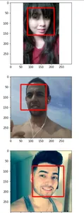
We visualize the bounding boxes predicted by the Bbox regressor for some images in the test set by drawing the bounding boxes in the images.

for inputs, labels in test_dataset:
    bbox_preds = bbox_regressor(inputs, training=False).numpy() 
    bbox_preds = (bbox_preds * (dataset_generator.target_shape * 2)).astype(int)
    imgs = (127 * (inputs + 1)).numpy().astype(np.uint8)
    for idx, img in enumerate(imgs):
        x1, y1, x2, y2 = bbox_preds[idx]
        img = cv2.rectangle(img, (x1, y1), (x2, y2), (255, 0, 0), 4)
        plt.imshow(img)
        plt.show()
    break

Output

Conclusion

In conclusion, CNN-based localizers are instrumental in advancing computer vision applications, particularly in object localization tasks. The article highlighted the importance of CNNs in image analysis and explained the two-step pipeline, involving a backbone CNN for feature extraction and a regression head for predicting bounding box coordinates. The future of object localization holds immense potential with advancements in deep learning techniques, larger datasets, and integration of other modalities, promising significant impacts on industries and transforming visual perception and understanding.

Key Takeaways

• CNN-based localizers are essential for advancing computer vision applications, leveraging CNNs’ ability to learn hierarchical features from images.
• The two-step pipeline, consisting of a feature extraction backbone CNN and a regression head, is commonly used in CNN-based localizers to achieve accurate object localization.
• The future of object localization holds great promise with advancements in deep learning, larger datasets, and the integration of other modalities, offering significant impacts on industries such as autonomous driving, robotics, surveillance, and healthcare.

The media shown in this article is not owned by Analytics Vidhya and is used at the Author’s discretion.

Babina Banjara 17 Aug 2023