Market Basket Analysis Based on RFM Analysis
This article was published as a part of the Data Science Blogathon.
Introduction on RFM Analysis
RFM and Market Basket Analysis is one of the applications of machine learning in the ecommerce and retail sector. Nowadays the machine learnings algorithms are playing a crucial role to enable the retail and ecommerce market to enhance their top and bottom line of business. This article will take you through the process of finding the frequently bought products together by the customers by analysing their past buying behaviour and segmenting them into different customer segments. This customer segments are formed on the basis of their buying patterns with respect to the recency, frequency and monetary parameters.

Customer Segmentation is the most critical subdivision of Marketing. Without segmenting a company’s customer, the marketing efforts can go haywire and lots of efforts and money is lost on the way. The best way to earn profits is to give your customer what he truly desires rather than the entire clutter. And after that also offer better choices of products based on his earlier purchases. This is a sure shot way of retaining a customer and making them feel like their needs are being heard and met.
Customers can be segmented in various ways like demographic, geographic, behavioural, psychographic etc. In this project the behavioural segmentation is targeted and customer’s behaviour and buying patterns are identified which are then used for personalized recommendations of the products. For doing this RFM Analysis and K-means clustering is used and the clusters formed have been used as a basis for Market Basket Analysis using Apriori Algorithm and compared with Item based collaborative filtering Algorithm.
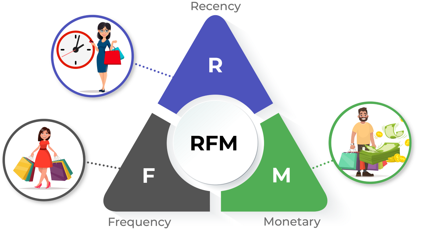
RFM analysis is the Recency, Frequency, Monetary Analysis in Marketing Analytics where the ‘R’ factor is about when was the last time a customer made a purchase, the ‘F’ factor is about the number of purchases made in a given period and ‘M’ factor is the total amount of money spent by the customer in the given time. The customers are grouped based on RFM values and assigned a RFM score. They are grouped into categories like ‘Gold’, ‘Silver’, ‘Bronze’ according to the RFM score.
Similarly in K-means clustering the RFM values are scaled and normalised and Elbow method is used to find the number of clusters or groups. Snake plots of both the techniques and have been drawn for a better comparison.
Market Basket Analysis is a proven data mining technique used for finding products brought together and in turn finding customer purchasing patterns and customer segments. New data frames based on RFM clusters have been created and Market Basket Analysis has been applied on the data frame using Apriori Algorithm which is a form of association rule mining that helps identify frequent item sets. Rules are formed and products having 70% confidence that will be purchased together are given as recommendations. Similarly, item based collaborative filtering is used to find the recommendations, the difference being the filtration based on correlation matrix. Both the algorithms are compared in the end and conclusions are drawn.
Objective
To compare the market Apriori Algorithm and Item Based Collaborative Filtering.
Provide customized recommendations to customer based on customer segmentation derived from RFM analysis.
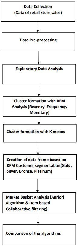
Flow of Tutorial
The figure below shows the major steps in the entire code to perform Market Basket Analysis on the basis of RFM analysis.
Data Overview
This is a transactions-based data set which contains all the transactions occurring for a year for a UK-based, registered non-store online retail. The company mainly sells various gift items. It has various attributes like the Quantity, Invoice number, Description of the product,Invoice date, Customer ID, Country, etc. It is a large dataset with over 5,20,000 records.
# import library
import numpy as np # linear algebra
import pandas as pd # data processing, CSV file I/O (e.g. pd.read_csv)
import datetime as dt
#For Data  Visualization
import matplotlib.pyplot as plt
import seaborn as sns
#For Machine Learning Algorithm
from sklearn.preprocessing import StandardScaler
from sklearn.cluster import KMeans
import os
df = pd.read_excel(r'D:ProjectFinal year project dataset.xlsx')
Data Pre-processing
It is very important to perform data pre-processing in order to make it suitable for further analysis. Quantity and Unit price column were found to have negative values which cannot be the case as these values are never negative in real life. Therefore rows having such entries were removed. In some cases the customer ID or Description was found to be missing. It could be matched to the stock code and filled the value but the unit price for these rows was found to be missing as well hence they were deleted. Even after deletion of all these rows some customer ID were still missing and were replaced by the customer Id from the data frame. This will not affect our market basket analysis. Also, rows with same stock code but different descriptions were fixed as this a common manual error.
df.head(5)
df.isnull().sum()
InvoiceNo 0
StockCode 0
Description 1454
Quantity 0
InvoiceDate 0
UnitPrice 0
CustomerID 135080
Country 0
dtype: int64
df= df.dropna(subset=['CustomerID'])
df.isnull().sum().sum()
0
#check and clean duplicate data
df.duplicated().sum()
5225
df = df.drop_duplicates()
df.duplicated().sum()
0
df.describe()
from datetime import datetime
from datetime import timedelta
convert_dict = {'InvoiceDate': str}
df = df.astype(convert_dict)
print(df.dtypes)
InvoiceNo object
StockCode object
Description object
Quantity int64
InvoiceDate object
UnitPrice float64
CustomerID float64
Country object
dtype: object
Here it was needed to have independent column of order date and order time to perform exploratory data analysis. This enabled us to find the day or month with highest sales and also the peak time of the day.
df['InvoiceDate']= pd.to_datetime(df['InvoiceDate'])
df['order_date'] = [d.date() for d in df['InvoiceDate']]
df['order_time'] = [d.time() for d in df['InvoiceDate']]
df.head()
df['order_date']= pd.to_datetime(df['order_date'])
date = datetime.strptime('2018-11-10 10:55:31', '%Y-%m-%d %H:%M:%S')
There are rows with unit price or quantitiy with values less than or equal to 0. But this is impossible in real life scenario. Therefore we eliminate such entries.
df=df[(df['Quantity']>0) & (df['UnitPrice']>0)]
df.describe()
The RFM values can be grouped in several ways. We are going to implement percentile-based grouping.
#New Total Sum Column
df['TotalSum'] = df['UnitPrice']* df['Quantity']
#Data preparation steps
print('Min Invoice Date:',df.order_date.dt.date.min(),'max Invoice Date:',
       df.order_date.dt.date.max())
df.head(3)
snapshot_date = df['order_date'].max() + dt.timedelta(days=1)

snapshot_date

#The last day of purchase in total is 09 DEC, 2011. To calculate the day periods,

#let's set one day after the last one,or

#10 DEC as a snapshot_date. We will cound the diff days with snapshot_date.
Calculate RFM Metrics
rfm = df.groupby(['CustomerID']).agg({'order_date': lambda x : (snapshot_date - x.max()).days,

'InvoiceNo':'count','TotalSum': 'sum'})
Function Lambda gives the number of days between hypothetical today and the last transaction
Rename columns
rfm.rename(columns={'order_date':'Recency','InvoiceNo':'Frequency',
'TotalSum':'MonetaryValue'},inplace= True)
#Final RFM values
rfm.head()
Note:
We will rate “Recency” customer who have been active more recently better than the less recent customer, because each company wants its customers to be recent.
We will rate “Frequency” and “Monetary Value” higher label because we want customer to spend more money and visit more often (that is different order than recency).
Building RFM Segments
r_labels =range(4,0,-1)

f_labels=range(1,5)

m_labels=range(1,5)

r_quartiles = pd.qcut(rfm['Recency'], q=4, labels = r_labels)

f_quartiles = pd.qcut(rfm['Frequency'],q=4, labels = f_labels)

m_quartiles = pd.qcut(rfm['MonetaryValue'],q=4,labels = m_labels)

rfm = rfm.assign(R=r_quartiles,F=f_quartiles,M=m_quartiles)

# Build RFM Segment and RFM Score

def add_rfm(x) : return str(x['R']) + str(x['F']) + str(x['M'])

rfm['RFM_Segment'] = rfm.apply(add_rfm,axis=1 )

rfm['RFM_Score'] = rfm[['R','F','M']].sum(axis=1)

rfm.head()
Analyzing RFM Segments
It is always the best practice to investigate the size of the segments before you use them for targeting or other business application.
rfm.groupby(['RFM_Segment']).size().sort_values(ascending=False)[:5]
RFM_Segment
4.04.04.0 443
1.01.01.0 381
3.04.04.0 222
1.02.02.0 206
2.01.01.0 181
dtype: int64
Summary metrics per RFM Score
rfm.groupby('RFM_Score').agg({'Recency': 'mean','Frequency': 'mean',

'MonetaryValue': ['mean', 'count'] }).round(1)
Use RFM score to group customers into gold, silver and bronze segments:
def segments(df):

if df['RFM_Score'] > 9 :

return 'Gold'

elif (df['RFM_Score'] > 5) and (df['RFM_Score'] <= 9 ):

return 'Silver'

else:

return 'Bronze'

rfm['General_Segment'] = rfm.apply(segments,axis=1)

rfm.groupby('General_Segment').agg({'Recency':'mean','Frequency':'mean',

'MonetaryValue':['mean','count']}).round(1)
Merged rfm and main dataframe
mdf=pd.merge(df,rfm,on='CustomerID')

mdf
Created 3 data frames based on RFM segments to perform MBA.
Bronze_seg = mdf[mdf.General_Segment == 'Bronze']

Bronze_seg

Silver_seg = mdf[mdf.General_Segment == 'Bronze']

Silver_seg

Gold_seg = mdf[mdf.General_Segment == 'Bronze']

Gold_seg
Data Pre-Processing for K-means Clustering
We must check these Key k-means assumptions before we implement our K-means clustering Mode
- Symmetric distribution of variables (not skewed)
- Variables with same average values
- Variables with same variance
rfm_rfm = rfm[['Recency','Frequency','MonetaryValue']]
print(rfm_rfm.describe())
From this table, we find this problem: Mean and Variance are not Equal
Solution: Scaling variables by using a scaler from scikit-learn library
Plot the distribution of RFM values
f,ax = plt.subplots(figsize=(10, 12))

plt.subplot(3, 1, 1); sns.distplot(rfm.Recency, label = 'Recency')

plt.subplot(3, 1, 2); sns.distplot(rfm.Frequency, label = 'Frequency')

plt.subplot(3, 1, 3); sns.distplot(rfm.MonetaryValue, label = 'Monetary Value')

plt.style.use('fivethirtyeight')

plt.tight_layout()

plt.show()
Also, there is another Problem: Unsymmetric distribution of variables (Data skewed)
Solution: Logarithmic transformation (positive values only) will manage skewness
We use these Sequence of structuring pre-processing steps:
1. Unskew the data – log transformation
2. Standardize to the same average values
3. Scale to the same standard deviation
4. Store as a separate array to be used for clustering
Why the Sequence Matters?
- Log transformation only works with positive data
- Normalization forces data to have negative values and log will not work
Unskew the data with log transformation
rfm_log = rfm[['Recency', 'Frequency', 'MonetaryValue']].apply(np.log, axis = 1).round(3)
#or rfm_log = np.log(rfm_rfm)
# plot the distribution of RFM values
f,ax = plt.subplots(figsize=(10, 12))
plt.subplot(3, 1, 1); sns.distplot(rfm_log.Recency, label = 'Recency')
plt.subplot(3, 1, 2); sns.distplot(rfm_log.Frequency, label = 'Frequency')
plt.subplot(3, 1, 3); sns.distplot(rfm_log.MonetaryValue, label = 'Monetary Value')
plt.style.use('fivethirtyeight')
plt.tight_layout()
plt.show()
Implementation of K-Means Clustering
#Normalize the variables with StandardScaler
from sklearn.preprocessing import StandardScaler
scaler = StandardScaler()
scaler.fit(rfm_log)
#Store it separately for clustering
rfm_normalized= scaler.transform(rfm_log)
Choosing no of Clusters
from sklearn.cluster import KMeans
#First : Get the Best KMeans
ks = range(1,8)
inertias=[]
for k in ks :
    # Create a KMeans clusters
    kc = KMeans(n_clusters=k,random_state=1)
    kc.fit(rfm_normalized)
    inertias.append(kc.inertia_)
# Plot ks vs inertias
f, ax = plt.subplots(figsize=(15, 8))
plt.plot(ks, inertias, '-o')
plt.xlabel('Number of clusters, k')
plt.ylabel('Inertia')
plt.xticks(ks)
plt.style.use('ggplot')
plt.title('What is the Best Number for KMeans ?')
plt.show()
Clustering
kc = KMeans(n_clusters= 3, random_state=1)

kc.fit(rfm_normalized)

#Create a cluster label column in the original DataFrame

cluster_labels = kc.labels_

#Calculate average RFM values and size for each cluster:

rfm_rfm_k3 = rfm_rfm.assign(K_Cluster = cluster_labels)

#Calculate average RFM values and sizes for each cluster:

rfm_rfm_k3.groupby('K_Cluster').agg({'Recency': 'mean','Frequency': 'mean',

                                         'MonetaryValue': ['mean', 'count'],}).round(0)
Snake Plots to Understand and Compare Segments
- Market research technique to compare different segments
- Visual representation of each segment’s attributes
- Need to first normalize data (center & scale)
- Plot each cluster’s average normalized values of each attribute
rfm_normalized = pd.DataFrame(rfm_normalized,index=rfm_rfm.index,columns=rfm_rfm.columns)

rfm_normalized['K_Cluster'] = kc.labels_

rfm_normalized['General_Segment'] = rfm['General_Segment']

rfm_normalized.reset_index(inplace = True)

#Melt the data into a long format so RFM values and metric names are stored in 1 column each

rfm_melt = pd.melt(rfm_normalized,id_vars=['CustomerID','General_Segment','K_Cluster'],

                            value_vars=['Recency', 'Frequency', 'MonetaryValue'],

var_name='Metric',value_name='Value')

var_name='Metric',value_name='Value')

rfm_melt.head()
Snake Plot
f, (ax1, ax2) = plt.subplots(1,2, figsize=(15, 8))

sns.lineplot(x = 'Metric', y = 'Value', hue = 'General_Segment', data = rfm_melt,ax=ax1)

# a snake plot with K-Means

sns.lineplot(x = 'Metric', y = 'Value', hue = 'K_Cluster', data = rfm_melt,ax=ax2)

plt.suptitle("Snake Plot of RFM",fontsize=24) #make title fontsize subtitle

plt.show()
Market Basket Analysis
Apriori Algorithm
Apriori algorithm works on the principle of how two or more products/objects are associated with each other. In orther words, we can say that it is an algorithm that analyzes customers who bought product A also bought product B. Generally it works on datasets containing large number of transactions.
basket_bronze = (Bronze_seg.groupby(['InvoiceNo', 'Description'])['Quantity']

          .sum().unstack().reset_index().fillna(0)

          .set_index('InvoiceNo'))

basket_bronze.head()

basket_bronze.copy = basket_bronze

basket_bronze.copy.head()


basket_bronze.copy = basket_bronze.copy.astype(int)


basket_bronze.copy.shape

(1711, 2831)


def encode_units(x):

    if x <= 0:

        return 0

    if x >= 1:

        return 1

basket_bronze_sets = basket_bronze.copy.applymap(encode_units)

basket_bronze_sets.drop('POSTAGE', inplace=True, axis=1)

basket_bronze_sets.head()
Import necessary libraries required for market basket analysis
from mlxtend.frequent_patterns import apriori

from mlxtend.frequent_patterns import association_rules

%matplotlib inline


frequent_itemsets_bronze = apriori(basket_bronze_sets, min_support=0.03, use_colnames=True)

#Build frequent itemsets

frequent_itemsets_bronze['length'] = frequent_itemsets_bronze['itemsets'].apply(lambda x: len(x))

frequent_itemsets_bronze


rules_bronze = association_rules(frequent_itemsets_bronze, metric="lift", min_threshold=1)

rules_bronze


#Products having 70% confidence likely to be purchased together

rules_bronze[(rules_bronze['lift'] >= 6) & (rules_bronze['confidence'] >= 0.7)]
Item Based Collaborative Filtering for Bronze Segment
It is an approach to predict the customers’ choice and find the products that customers might tend to buy on the basis of the data collected from a large number of different customers having similar choices or preferences. The basic consideration is that if person A and person B have some kind of reaction to some items, then they might have the same preferences or opinion towards other items too.
Co-occurence Matrix
CID_PN_matrix = Bronze_seg.pivot_table(index = ["InvoiceNo"], columns = ["Description"],

                              values = "Quantity").fillna(0)

basket_bronze_set = CID_PN_matrix.applymap(encode_units)

basket_bronze_set_int = basket_bronze_set.astype(int)

coocM_Bronze = basket_bronze_set_int.T.dot(basket_bronze_set_int)

x_Bronze = pd.DataFrame(coocM_Bronze.idxmax()).reset_index()

x_Bronze.columns = ["A", "B"]

x_Bronze

r_Bronze = x_Bronze[x_Bronze["A"] != x_Bronze["B"]]

r_Bronze.head(10)

matrix_Bronze = Bronze_seg.pivot_table(index = ["InvoiceNo"], columns = ["Description"],

                              values = "Quantity")

matrix_Bronze.head(10)

whiteHeart = matrix_Bronze["WHITE HANGING HEART T-LIGHT HOLDER"]

whiteHeart.head()

InvoiceNo
536374   NaN
536384   NaN
536388   NaN
536393   NaN
536403   NaN
Name: WHITE HANGING HEART T-LIGHT HOLDER, dtype: float64

similarProductsW_Bronze = matrix_Bronze.corrwith(whiteHeart)

similarProductsW_Bronze = similarProductsW_Bronze.dropna()

df1 = pd.DataFrame(similarProductsW_Bronze)

df1.head(10)

corrMatrix_Bronze = matrix_Bronze.corr()

corrMatrix_Bronze.head()

second_customer_Bronze = matrix_Bronze.iloc[1].dropna()

second_customer_Bronze.head()

Description
CLASSIC METAL BIRDCAGE PLANT HOLDER 2.0
COLOUR GLASS T-LIGHT HOLDER HANGING 48.0
CREAM HEART CARD HOLDER 4.0
ENAMEL BREAD BIN CREAM 8.0
ENAMEL FIRE BUCKET CREAM 6.0
Name: 536384, dtype: float64

simProducts_Bronze = pd.Series()

#Go through every product bought by second customer

for i in range(0, len(second_customer_Bronze.index)):

    print("Adding sims for " + second_customer_Bronze.index[i] + "....")

    #Retrieve similar products to the ones bought by customer 2

    sims_Bronze = corrMatrix_Bronze[second_customer_Bronze.index[i]].dropna()

    #Scale to how many of the products were bought

    sims_Bronze = sims_Bronze.map(lambda x: x * second_customer_Bronze[i])

    # Add to the list of similar products

    simProducts_Bronze = simProducts_Bronze.append(sims_Bronze)

print("sorting...")

simProducts_Bronze.sort_values(inplace = True, ascending = True)

print(simProducts_Bronze)

Sorting the results and avoiding duplicates
simProducts_Bronze= simProducts_Bronze.groupby(simProducts_Bronze.index).sum().

                                            sort_values(ascending = False)

filteredSims_Bronze = simProducts_Bronze.drop(second_customer_Bronze.index)

filteredSims_Bronze.head(5)

CANDLEHOLDER PINK HANGING HEART       148.831186
METAL 4 HOOK HANGER FRENCH CHATEAU    138.851682
ROSES REGENCY TEACUP AND SAUCER       129.773943
GREEN REGENCY TEACUP AND SAUCER       128.413480
SINGLE ANTIQUE ROSE HOOK IVORY        128.000000
dtype: float64
In this way you need to run the Apriori algorithm as well as Item based collaborative filtering algorithm for other segments to provide customised recommendations to the customer from those segments.
Comparison of Algorithms
After running the algorithm for all the segments, this analysis shows that as the support values decreases or move towards less than or equal to 0.01, sometimes Apriori Algorithm fails to generate the frequent patterns as it gets involved in infinite loop. Also, as minimum support increases the frequent item set generated decreases.
To generate association rules for such heavy datasets, all the algorithms have different run-time due to their unique execution processes. As per the analysis, Apriori was efficient in terms of run-time. IBCF took a long time. It was observed that the execution time for Item based collaborative filtering was 840 seconds and for Apriori algorithm was 480 seconds
Conclusion on RFM Analysis
In this tutorial we have learned about the Apriori algorithm and item based collaborative filtering and how it is coupled with RFM analysis to generate personalized recommendations based on customer’s segment which is associated his buying behaviour. The code is designed in such a way that it enables you to first implement RFM analysis and compare those segments with clusters formed using K Means Clustering. Further we have executed Market Basket Analysis for Bronze segment.
I hope this tutorial gave you overview of the RFM analysis and market basket analysis and its implementation using python.
The media shown in this article is not owned by Analytics Vidhya and is used at the Author’s discretion.


