Practical Guide on Data Preprocessing in Python using Scikit Learn
Introduction
This article primarily focuses on data pre-processing techniques in python. Learning algorithms have affinity towards certain data types on which they perform incredibly well. They are also known to give reckless predictions with unscaled or unstandardized features. Algorithm like XGBoost, specifically requires dummy encoded data while algorithm like decision tree doesn’t seem to care at all (sometimes)!
In simple words, pre-processing refers to the transformations applied to your data before feeding it to the algorithm. In python, scikit-learn library has a pre-built functionality under sklearn.preprocessing. There are many more options for pre-processing which we’ll explore.
After finishing this article, you will be equipped with the basic techniques of data pre-processing and their in-depth understanding. For your convenience, I’ve attached some resources for in-depth learning of machine learning algorithms and designed few exercises to get a good grip of the concepts.

Available Data set
For this article, I have used a subset of the Loan Prediction (missing value observations are dropped) data set from You can download the final training and testing data set from here: Download Data
Note : Testing data that you are provided is the subset of the training data from Loan Prediction problem.
Now, lets get started by importing important packages and the data set.
# Importing pandas
>> import pandas as pd
# Importing training data set
>> X_train=pd.read_csv('X_train.csv')
>> Y_train=pd.read_csv('Y_train.csv')
# Importing testing data set
>> X_test=pd.read_csv('X_test.csv')
>> Y_test=pd.read_csv('Y_test.csv')
Lets take a closer look at our data set.
>> print (X_train.head())
Feature Scaling
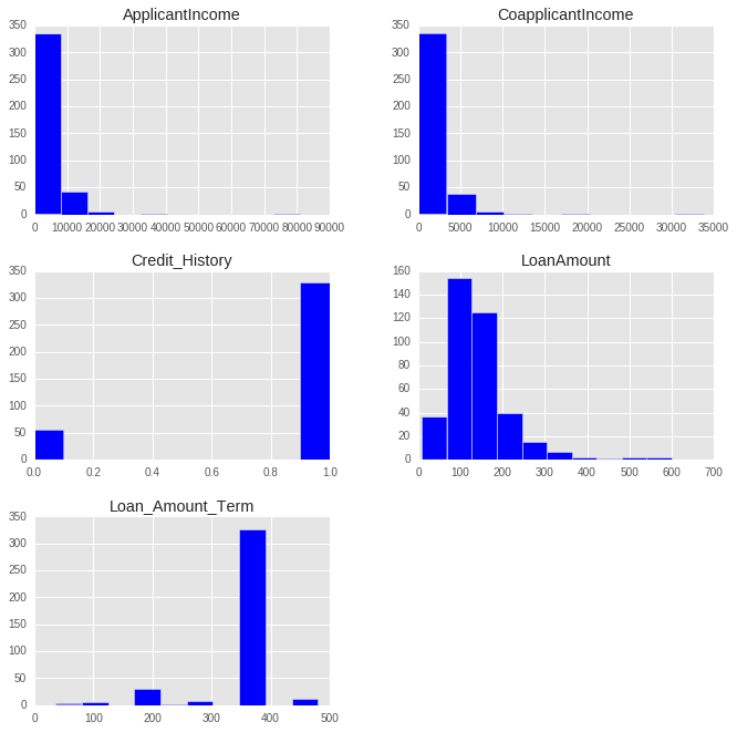
Feature scaling is the method to limit the range of variables so that they can be compared on common grounds. It is performed on continuous variables. Lets plot the distribution of all the continuous variables in the data set.
>> import matplotlib.pyplot as plt
>> X_train[X_train.dtypes[(X_train.dtypes=="float64")|(X_train.dtypes=="int64")]
                        .index.values].hist(figsize=[11,11])
# Importing MinMaxScaler and initializing it
>> from sklearn.preprocessing import MinMaxScaler
>> min_max=MinMaxScaler()
# Scaling down both train and test data set
>> X_train_minmax=min_max.fit_transform(X_train[['ApplicantIncome', 'CoapplicantIncome',
                'LoanAmount', 'Loan_Amount_Term', 'Credit_History']])
>> X_test_minmax=min_max.fit_transform(X_test[['ApplicantIncome', 'CoapplicantIncome',
                'LoanAmount', 'Loan_Amount_Term', 'Credit_History']])
# Fitting k-NN on our scaled data set
>> knn=KNeighborsClassifier(n_neighbors=5)
>> knn.fit(X_train_minmax,Y_train)
# Checking the model's accuracy
>> accuracy_score(Y_test,knn.predict(X_test_minmax))
Out : 0.75
Exercise 1
Try to do the same exercise with a logistic regression model(parameters : penalty=’l2′,C=0.01) and provide your accuracy before and after scaling in the comment section.
Feature Standardization
Before jumping to this section I suggest you to complete Exercise 1.
In the previous section, we worked on the Loan_Prediction data set and fitted a kNN learner on the data set. After scaling down the data, we have got an accuracy of 75% which is very considerably good. I tried the same exercise on Logistic Regression and I got the following result :
Before Scaling : 61%
After Scaling : 63%
The accuracy we got after scaling is close to the prediction which we made by guessing, which is not a very impressive achievement. So, what is happening here? Why hasn’t the accuracy increased by a satisfactory amount as it increased in kNN?
Resources : Go through this article on Logistic Regression for better understanding.
Here is the answer:
In logistic regression, each feature is assigned a weight or coefficient (Wi). If there is a feature with relatively large range and it is insignificant in the objective function then logistic regression will itself assign a very low value to its co-efficient, thus neutralizing the dominant effect of that particular feature, whereas distance based method such as kNN does not have this inbuilt strategy, thus it requires scaling.
Aren’t we forgetting something ? Our logistic model is still predicting with an accuracy almost closer to a guess.
Now, I’ll be introducing a new concept here called standardization. Many machine learning algorithms in sklearn requires standardized data which means having zero mean and unit variance.
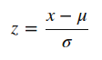
Standardization (or Z-score normalization) is the process where the features are rescaled so that they’ll have the properties of a standard normal distribution with μ=0 and σ=1, where μ is the mean (average) and σ is the standard deviation from the mean. Standard scores (also called z scores) of the samples are calculated as follows :
Elements such as l1 ,l2 regularizer in linear models (logistic comes under this category) and RBF kernel in SVM in objective function of learners assumes that all the features are centered around zero and have variance in the same order.
Features having larger order of variance would dominate on the objective function as it happened in the previous section with the feature having large range. As we saw in the Exercise 1 that without any preprocessing on the data the accuracy was 61%, lets standardize our data apply logistic regression on that. Sklearn provides scale to standardize the data.
# Standardizing the train and test data
>> from sklearn.preprocessing import scale
>> X_train_scale=scale(X_train[['ApplicantIncome', 'CoapplicantIncome',
                'LoanAmount', 'Loan_Amount_Term', 'Credit_History']])
>> X_test_scale=scale(X_test[['ApplicantIncome', 'CoapplicantIncome',
               'LoanAmount', 'Loan_Amount_Term', 'Credit_History']])
# Fitting logistic regression on our standardized data set
>> from sklearn.linear_model import LogisticRegression
>> log=LogisticRegression(penalty='l2',C=.01)
>> log.fit(X_train_scale,Y_train)
# Checking the model's accuracy
>> accuracy_score(Y_test,log.predict(X_test_scale))
Out : 0.75
We again reached to our maximum score that was attained using kNN after scaling. This means standardizing the data when using a estimator having l1 or l2 regularization helps us to increase the accuracy of the prediction model. Other learners like kNN with euclidean distance measure, k-means, SVM, perceptron, neural networks, linear discriminant analysis, principal component analysis may perform better with standardized data.
Though, I suggest you to understand your data and what kind of algorithm you are going to apply on it; over the time you will be able to judge weather to standardize your data or not.
Note : Choosing between scaling and standardizing is a confusing choice, you have to dive deeper in your data and learner that you are going to use to reach the decision. For starters, you can try both the methods and check cross validation score for making a choice.
Resources : Go through this article on cross validation for better understanding.
Exercise 2
Try to do the same exercise with SVM model and provide your accuracy before and after standardization in the comment section.
Resources : Go through this article on support vector machines for better understanding.
Label Encoding
In previous sections, we did the pre-processing for continuous numeric features. But, our data set has other features too such as Gender, Married, Dependents, Self_Employed and Education. All these categorical features have string values. For example, Gender has two levels either Male or Female. Lets feed the features in our logistic regression model.
# Fitting a logistic regression model on whole data
>> log=LogisticRegression(penalty='l2',C=.01)
>> log.fit(X_train,Y_train)
# Checking the model's accuracy
>> accuracy_score(Y_test,log.predict(X_test))
Out : ValueError: could not convert string to float: Semiurban
We got an error saying that it cannot convert string to float. So, what’s actually happening here is learners like logistic regression, distance based methods such as kNN, support vector machines, tree based methods etc. in sklearn needs numeric arrays. Features having string values cannot be handled by these learners.
Sklearn provides a very efficient tool for encoding the levels of a categorical features into numeric values. LabelEncoder encode labels with value between 0 and n_classes-1.
Lets encode all the categorical features.
# Importing LabelEncoder and initializing it
>> from sklearn.preprocessing import LabelEncoder
>> le=LabelEncoder()
# Iterating over all the common columns in train and test
>> for col in X_test.columns.values:
       # Encoding only categorical variables
       if X_test[col].dtypes=='object':
       # Using whole data to form an exhaustive list of levels
       data=X_train[col].append(X_test[col])
       le.fit(data.values)
       X_train[col]=le.transform(X_train[col])
       X_test[col]=le.transform(X_test[col])
All our categorical features are encoded. You can look at your updated data set using X_train.head(). We are going to take a look at Gender frequency distribution before and after the encoding.
Before : Male 318
         Female 66
Name: Gender, dtype: int64
After : 1 318
        0 66
Name: Gender, dtype: int64
Now that we are done with label encoding, lets now run a logistic regression model on the data set with both categorical and continuous features.
# Standardizing the features
>> X_train_scale=scale(X_train)
>> X_test_scale=scale(X_test)
# Fitting the logistic regression model
>> log=LogisticRegression(penalty='l2',C=.01)
>> log.fit(X_train_scale,Y_train)
# Checking the models accuracy
>> accuracy_score(Y_test,log.predict(X_test_scale))
Out : 0.75
Its working now. But, the accuracy is still the same as we got with logistic regression after standardization from numeric features. This means categorical features we added are not very significant in our objective function.
Exercise 3
Try out decision tree classifier with all the features as independent variables and comment your accuracy.
Resources : Go through this article on decision trees for better understanding.
One-Hot Encoding
One-Hot Encoding transforms each categorical feature with n possible values into n binary features, with only one active.
Most of the ML algorithms either learn a single weight for each feature or it computes distance between the samples. Algorithms like linear models (such as logistic regression) belongs to the first category.
Lets take a look at an example from loan_prediction data set. Feature Dependents have 4 possible values 0,1,2 and 3+ which are then encoded without loss of generality to 0,1,2 and 3.
We, then have a weight “W” assigned for this feature in a linear classifier,which will make a decision based on the constraints W*Dependents + K > 0 or eqivalently W*Dependents < K.
Let f(w)= W*Dependents
Possible values that can be attained by the equation are 0, W, 2W and 3W. A problem with this equation is that the weight “W” cannot make decision based on four choices. It can reach to a decision in following ways:
- All leads to the same decision (all of them <K or vice versa)
- 3:1 division of the levels (Decision boundary at f(w)>2W)
- 2:2 division of the levels (Decision boundary at f(w)>W)
Here we can see that we are loosing many different possible decisions such as the case where “0” and “2W” should be given same label and “3W” and “W” are odd one out.
This problem can be solved by One-Hot-Encoding as it effectively changes the dimensionality of the feature “Dependents” from one to four, thus every value in the feature “Dependents” will have their own weights. Updated equation for the decison would be f'(w) < K.
where, f'(w) = W1*D_0 + W2*D_1 + W3*D_2 + W4*D_3All four new variable has boolean values (0 or 1).
The same thing happens with distance based methods such as kNN. Without encoding, distance between “0” and “1” values of Dependents is 1 whereas distance between “0” and “3+” will be 3, which is not desirable as both the distances should be similar. After encoding, the values will be new features (sequence of columns is 0,1,2,3+) : [1,0,0,0] and [0,0,0,1] (initially we were finding distance between “0” and “3+”), now the distance would be √2.
For tree based methods, same situation (more than two values in a feature) might effect the outcome to extent but if methods like random forests are deep enough, it can handle the categorical variables without one-hot encoding.
Now, lets take look at the implementation of one-hot encoding with various algorithms.
Lets create a logistic regression model for classification without one-hot encoding.
# We are using scaled variable as we saw in previous section that
# scaling will effect the algo with l1 or l2 reguralizer
>> X_train_scale=scale(X_train)
>> X_test_scale=scale(X_test)
# Fitting a logistic regression model
>> log=LogisticRegression(penalty='l2',C=1)
>> log.fit(X_train_scale,Y_train)
# Checking the model's accuracy
>> accuracy_score(Y_test,log.predict(X_test_scale))
Out : 0.73958333333333337
Now we are going to encode the data.
>> from sklearn.preprocessing import OneHotEncoder
>> enc=OneHotEncoder(sparse=False)
>> X_train_1=X_train
>> X_test_1=X_test
>> columns=['Gender', 'Married', 'Dependents', 'Education','Self_Employed',
          'Credit_History', 'Property_Area']
>> for col in columns:
       # creating an exhaustive list of all possible categorical values
       data=X_train[[col]].append(X_test[[col]])
       enc.fit(data)
       # Fitting One Hot Encoding on train data
       temp = enc.transform(X_train[[col]])
       # Changing the encoded features into a data frame with new column names
       temp=pd.DataFrame(temp,columns=[(col+"_"+str(i)) for i in data[col]
            .value_counts().index])
       # In side by side concatenation index values should be same
       # Setting the index values similar to the X_train data frame
       temp=temp.set_index(X_train.index.values)
       # adding the new One Hot Encoded varibales to the train data frame
       X_train_1=pd.concat([X_train_1,temp],axis=1)
       # fitting One Hot Encoding on test data
       temp = enc.transform(X_test[[col]])
       # changing it into data frame and adding column names
       temp=pd.DataFrame(temp,columns=[(col+"_"+str(i)) for i in data[col]
            .value_counts().index])
       # Setting the index for proper concatenation
       temp=temp.set_index(X_test.index.values)
       # adding the new One Hot Encoded varibales to test data frame
       X_test_1=pd.concat([X_test_1,temp],axis=1)
Now, lets apply logistic regression model on one-hot encoded data.
# Standardizing the data set
>> X_train_scale=scale(X_train_1)
>> X_test_scale=scale(X_test_1)
# Fitting a logistic regression model
>> log=LogisticRegression(penalty='l2',C=1)
>> log.fit(X_train_scale,Y_train)
# Checking the model's accuracy
>> accuracy_score(Y_test,log.predict(X_test_scale))
Out : 0.75
Here, again we got the maximum accuracy as 0.75 that we have gotten so far. In this case, logistic regression regularization(C) parameter 1 where as earlier we used C=0.01.
End Notes
The aim of this article is to familiarize you with the basic data pre-processing techniques and have a deeper understanding of the situations of where to apply those techniques.
These methods work because of the underlying assumptions of the algorithms. This is by no means an exhaustive list of the methods. I’d encourage you to experiment with these methods since they can be heavily modified according to the problem at hand.
I plan to provide more advance techniques of data pre-processing such as pipeline and noise reduction in my next post, so stay tuned to dive deeper into the data pre-processing.
Did you like reading this article ? Do you follow a different approach / package / library to perform these talks. I’d love to interact with you in comments.
You can test your skills and knowledge. Check out Live Competitions and compete with best Data Scientists from all over the world.
I am Syed Danish, currently pursuing my bachelors in Electronics & Communication Engineering from ISM Dhanbad. I am a data science and machine learning enthusiast.


Useful...
Thanks for the post. It was useful to me!
Feature scaling code X_train[X_train.dtypes[(X_train.dtypes=="float64")|(X_train.dtypes=="int64")].index.values].hist(figsize=[11,11]) is not working. There is something wrong there.
There was some problem with the formatting of inverted commas, Thanks for bringing my attention towards it.
thanks a lot. .
This is also not working - accuracy_score(Y_test,knn.predict(X_test[['ApplicantIncome', 'CoapplicantIncome','LoanAmount', 'Loan_Amount_Term', 'Credit_History']])) Do you have working code?
Every line of code is tested. There is a problem with the formatting of the apostrophe(') when I copied your code from comment section, although it is working fine for me when I copied the code from the article. P.S. formatting of apostrophe and inverted commas are messing up the code, please check the formatting before running the code.
When typing: knn.fit(X_train[['ApplicantIncome', 'CoapplicantIncome','LoanAmount', 'Loan_Amount_Term', 'Credit_History']],Y_train) I received the following error: ValueError: Found arrays with inconsistent numbers of samples: [383 384] Do you know what's wrong?
Please download the data set again,there was a problem in it which has already been corrected.
####Exercise 1 Before Scaling accuracy 0.614583333333 After Scaling accuracy 0.635416666667 #### Exercise 2 before standardization 0.645833333333 after standardization 0.75 ####Exercise 3 before standardization accuracy 0.677083333333 after standardization accuracy 0.71875
It sounds right. Were you able to understand the jump(amount of jump also) in the accuracy of the given exercises for corresponding learning algorithm?
knn.fit(X_train[['ApplicantIncome', 'CoapplicantIncome','LoanAmount', 'Loan_Amount_Term', 'Credit_History']],Y_train) There seems to be some problem with the code. Can you please help me in rectifying the error. I am assuming it is python version error. knn.fit(X_train[['ApplicantIncome', 'CoapplicantIncome','LoanAmount', 'Loan_Amount_Term', 'Credit_History']],Y_train) Traceback (most recent call last): File "", line 2, in 'Loan_Amount_Term', 'Credit_History']],Y_train) File "/home/fractaluser/anaconda3/lib/python3.5/site-packages/sklearn/neighbors/base.py", line 792, in fit check_classification_targets(y) File "/home/fractaluser/anaconda3/lib/python3.5/site-packages/sklearn/utils/multiclass.py", line 170, in check_classification_targets y_type = type_of_target(y) File "/home/fractaluser/anaconda3/lib/python3.5/site-packages/sklearn/utils/multiclass.py", line 238, in type_of_target if is_multilabel(y): File "/home/fractaluser/anaconda3/lib/python3.5/site-packages/sklearn/utils/multiclass.py", line 154, in is_multilabel labels = np.unique(y) File "/home/fractaluser/anaconda3/lib/python3.5/site-packages/numpy/lib/arraysetops.py", line 198, in unique ar.sort() TypeError: unorderable types: int() > str()
Hi anit, I also think that there is a problem with the version of python as it is working fine on my machine(python 2.7), although after looking at the errors I suggest you to convert the outcome feature i.e, Y_train to numerics ('Y'=1 and 'N'=0). You can use label enoder for the same or use apply function. Let me know if this works out for you.
le.fit(data.values) This line is throwing an error . Please help ar.sort() TypeError: unorderable types: str() > float()
Hi Nishant, Check if you are using only the categorical variables for label encoding. If you still face this problem, send me the codes that you are using.
Many thanks very practical. Will certainly share site with my buddies
Thanks for the wonderful post. I have a question regarding the standardization: I read from the documentation of sklearn that the feature preprocessing should be learned from the training set and applied on the testing set, but in the post, the standardization was done as: >>X_train_scale=scale(X_train[['ApplicantIncome', 'CoapplicantIncome', 'LoanAmount', 'Loan_Amount_Term', 'Credit_History']]) >> X_test_scale=scale(X_test[['ApplicantIncome', 'CoapplicantIncome', 'LoanAmount', 'Loan_Amount_Term', 'Credit_History']]) According to my understanding, shouldn't it be something like: >>scaler = StandardScaler.fit(X_train[['ApplicantIncome', 'CoapplicantIncome', 'LoanAmount', 'Loan_Amount_Term', 'Credit_History']]) >>X_train_scale = scaler.transform(X_train[['ApplicantIncome', 'CoapplicantIncome', 'LoanAmount', 'Loan_Amount_Term', 'Credit_History']]) >> X_test_scale = scaler.transform(X_test[['ApplicantIncome', 'CoapplicantIncome', 'LoanAmount', 'Loan_Amount_Term', 'Credit_History']]) Please point out if my understanding is incorrect. Thanks a lot.
Hi Dai Zhongxiang, StandardScaler uses the Transformer API to compute the mean and standard deviation on a the data so as to be able to later reapply the transformation where as scale method provides quick way to perform the same operation. P.S. You can use both methods to perform the scaling operation.
Thank you. Very detailed and impressive article for beginners. How do we know which model use which standardization methods? For example, you use MinMaxScaler for kNN and Z-score for logistic regression, how about the other models? Is there any cheat sheet has the summary about this? Thank you again.
Hi Jack, thank you for your support. Using particular methods for a model mostly depends on observation but after learning the basics of algorithms and preprocessing methods you can get some idea about the type of method to use for a particular algorithm, As I mentioned in the article - "In logistic regression, each feature is assigned a weight or coefficient (Wi). If there is a feature with relatively large range and it is insignificant in the objective function then logistic regression will itself assign a very low value to its co-efficient, thus neutralizing the dominant effect of that particular feature, whereas distance based method such as kNN does not have this inbuilt strategy, thus it requires scaling." and also this section - " This means standardizing the data when using a estimator having l1 or l2 regularization helps us to increase the accuracy of the prediction model. Other learners like kNN with euclidean distance measure, k-means, SVM, perceptron, neural networks, linear discriminant analysis, principal component analysis may perform better with standardized data." Lastly it all come down to experience and deeper understanding. Hope this will help you understand the concepts more clearly.
Thank you for the post! I found it very helpful (I am new to Python). I have one question about the logistic regression in Exercise One. We are using the sklearn.linear_model for logistic regression. In this case, the decision boundary is a straight line. Is there a way to add some non-linearity the decision boundary?
Sir, how to assign weights to certain attributes in dataset as these attributes is more prominent in predicting
Very userful article
For K-neares neightbour implementation, why is there >> knn=KNeighborsClassifier(n_neighbors=5) Shouldn't n_neighbors=2 as there are two possible outcomes ?
hi... how the test and train files are extracted?
Very nice tutorial and I really like it so much! Have some suggestions : - We can apply both transformations (from text categories to integer categories, then from integer categories to one-hot vectors) in one shot using the LabelBinarizer class: Thanks
Hi syed, I noticed you did not drop the original columns after One-Hot encoding i.e columns=['Gender', 'Married', 'Dependents', 'Education','Self_Employed', 'Credit_History', 'Property_Area'] after X_train_1=pd.concat([X_train_1,temp],axis=1) Encoding created additional columns and the originals should be dropped. There might have been an increase in your accuracy if this step was taken. Very helpful post nonetheless
Excellent post.Loved the way you explained the process step by step. One small update to help newer users. For One-Hot encoding the latest release of Pandas has a new function called get_dummies(). It makes it super easy to do the encoding. Sample code below col = ['Gender', 'Married', 'Dependents', 'Education','Self_Employed','Credit_History', 'Property_Area'] X_train_dummy = pd.get_dummies(X_train, columns=col, drop_first=True) X_test_dummy = pd.get_dummies(X_test, columns=col, drop_first=True) Note: specify the columns, else it will only encode the categorical columns and drop the rest. Also, drop_first = True creates N-1 dummy variables which is the standard practice