Introduction to Feature Selection methods with an example (or how to select the right variables?)

Introduction

One of the best ways I use to learn machine learning is by benchmarking myself against the best data scientists in competitions. It gives you a lot of insight into how you perform against the best on a level playing field.

Initially, I used to believe that machine learning is going to be all about algorithms – know which one to apply when and you will come on the top. When I got there, I realized that was not the case – the winners were using the same algorithms which a lot of other people were using.

Next, I thought surely these people would have better / superior machines. I discovered that is not the case. I saw competitions being won using a MacBook Air, which is not the best computational machine. Over time, I realized that there are 2 things which distinguish winners from others in most of the cases: Feature Creation and Feature Selection.

In other words, it boils down to creating variables which capture hidden business insights and then making the right choices about which variable to choose for your predictive models! Sadly or thankfully, both these skills require a ton of practice. There is also some art involved in creating new features – some people have a knack of finding trends where other people struggle.

In this article, I will focus on one of the 2 critical parts of getting your models right – feature selection. I will discuss in detail why feature selection plays such a vital role in creating an effective predictive model.

If you are interested in exploring the concepts of feature engineering, feature selection and dimentionality reduction, check out the following comprehensive courses –

• Applied Machine Learning – Beginner to Professional
• Certified AI & ML Blackbelt+ Program

Read on!

Table of Contents

1. Importance of Feature Selection in Machine Learning
2. Filter Methods
3. Wrapper Methods
4. Embedded Methods
5. Difference between Filter and Wrapper methods
6. Walkthrough example

1. Importance of Feature Selection in Machine Learning

Machine learning works on a simple rule – if you put garbage in, you will only get garbage to come out. By garbage here, I mean noise in data.

This becomes even more important when the number of features are very large. You need not use every feature at your disposal for creating an algorithm. You can assist your algorithm by feeding in only those features that are really important. I have myself witnessed feature subsets giving better results than complete set of feature for the same algorithm. Or as Rohan Rao puts it – “Sometimes, less is better!”

Not only in the competitions but this can be very useful in industrial applications as well. You not only reduce the training time and the evaluation time, you also have less things to worry about!

Top reasons to use feature selection are:

• It enables the machine learning algorithm to train faster.
• It reduces the complexity of a model and makes it easier to interpret.
• It improves the accuracy of a model if the right subset is chosen.
• It reduces overfitting.

Next, we’ll discuss various methodologies and techniques that you can use to subset your feature space and help your models perform better and efficiently. So, let’s get started.

2. Filter Methods

Filter methods are generally used as a preprocessing step. The selection of features is independent of any machine learning algorithms. Instead, features are selected on the basis of their scores in various statistical tests for their correlation with the outcome variable. The correlation is a subjective term here. For basic guidance, you can refer to the following table for defining correlation co-efficients.

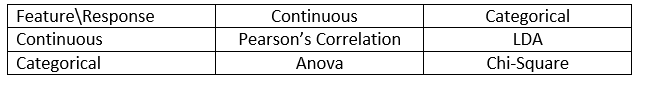
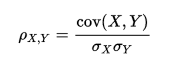
• Pearson’s Correlation: It is used as a measure for quantifying linear dependence between two continuous variables X and Y. Its value varies from -1 to +1. Pearson’s correlation is given as:

• LDA: Linear discriminant analysis is used to find a linear combination of features that characterizes or separates two or more classes (or levels) of a categorical variable.

• ANOVA: ANOVA stands for Analysis of variance. It is similar to LDA except for the fact that it is operated using one or more categorical independent features and one continuous dependent feature. It provides a statistical test of whether the means of several groups are equal or not.

• Chi-Square: It is a is a statistical test applied to the groups of categorical features to evaluate the likelihood of correlation or association between them using their frequency distribution.

One thing that should be kept in mind is that filter methods do not remove multicollinearity. So, you must deal with multicollinearity of features as well before training models for your data.

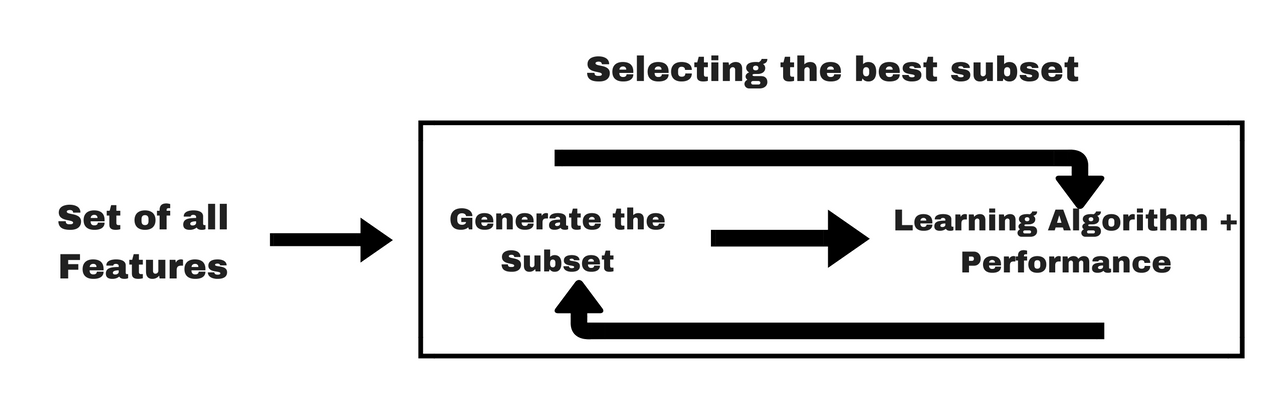
3. Wrapper Methods

In wrapper methods, we try to use a subset of features and train a model using them. Based on the inferences that we draw from the previous model, we decide to add or remove features from your subset. The problem is essentially reduced to a search problem. These methods are usually computationally very expensive.

Some common examples of wrapper methods are forward feature selection, backward feature elimination, recursive feature elimination, etc.

• Forward Selection: Forward selection is an iterative method in which we start with having no feature in the model. In each iteration, we keep adding the feature which best improves our model till an addition of a new variable does not improve the performance of the model.
• Backward Elimination: In backward elimination, we start with all the features and removes the least significant feature at each iteration which improves the performance of the model. We repeat this until no improvement is observed on removal of features.
• Recursive Feature elimination: It is a greedy optimization algorithm which aims to find the best performing feature subset. It repeatedly creates models and keeps aside the best or the worst performing feature at each iteration. It constructs the next model with the left features until all the features are exhausted. It then ranks the features based on the order of their elimination.

One of the best ways for implementing feature selection with wrapper methods is to use Boruta package that finds the importance of a feature by creating shadow features.

It works in the following steps:

1. Firstly, it adds randomness to the given data set by creating shuffled copies of all features (which are called shadow features).
2. Then, it trains a random forest classifier on the extended data set and applies a feature importance measure (the default is Mean Decrease Accuracy) to evaluate the importance of each feature where higher means more important.
3. At every iteration, it checks whether a real feature has a higher importance than the best of its shadow features (i.e. whether the feature has a higher Z-score than the maximum Z-score of its shadow features) and constantly removes features which are deemed highly unimportant.
4. Finally, the algorithm stops either when all features get confirmed or rejected or it reaches a specified limit of random forest runs.

For more information on the implementation of Boruta package, you can refer to this article :

For the implementation of Boruta in python, refer can refer to this article.

4. Embedded Methods

Embedded methods combine the qualities’ of filter and wrapper methods. It’s implemented by algorithms that have their own built-in feature selection methods.

Some of the most popular examples of these methods are LASSO and RIDGE regression which have inbuilt penalization functions to reduce overfitting.

• Lasso regression performs L1 regularization which adds penalty equivalent to absolute value of the magnitude of coefficients.
• Ridge regression performs L2 regularization which adds penalty equivalent to square of the magnitude of coefficients.

For more details and implementation of LASSO and RIDGE regression, you can refer to this article.

Other examples of embedded methods are Regularized trees, Memetic algorithm, Random multinomial logit.

5. Difference between Filter and Wrapper methods

The main differences between the filter and wrapper methods for feature selection are:

• Filter methods measure the relevance of features by their correlation with dependent variable while wrapper methods measure the usefulness of a subset of feature by actually training a model on it.
• Filter methods are much faster compared to wrapper methods as they do not involve training the models. On the other hand, wrapper methods are computationally very expensive as well.
• Filter methods use statistical methods for evaluation of a subset of features while wrapper methods use cross validation.
• Filter methods might fail to find the best subset of features in many occasions but wrapper methods can always provide the best subset of features.
• Using the subset of features from the wrapper methods make the model more prone to overfitting as compared to using subset of features from the filter methods.

6. Walkthrough example

Let’s use wrapper methods for feature selection and see whether we can improve the accuracy of our model by using an intelligently selected subset of features instead of using every feature at our disposal.

We’ll be using stock prediction data in which we’ll predict whether the stock will go up or down based on 100 predictors in R. This dataset contains 100 independent variables from X1 to X100 representing profile of a stock and one outcome variable Y with two levels : 1 for rise in stock price and -1 for drop in stock price.

To download the dataset, click here.

Let’s start with applying random forest for all the features on the dataset first.

library('Metrics')
library('randomForest')
library('ggplot2')
library('ggthemes')
library('dplyr')
#set random seed
set.seed(101)
#loading dataset
data<-read.csv("train.csv",stringsAsFactors= T)
#checking dimensions of data
dim(data)
## [1] 3000  101
#specifying outcome variable as factor
data$Y<-as.factor(data$Y)
data$Time<-NULL
#dividing the dataset into train and test
train<-data[1:2000,]
test<-data[2001:3000,]
#applying Random Forest
model_rf<-randomForest(Y ~ ., data = train)
preds<-predict(model_rf,test[,-101])
table(preds)
##preds
## -1   1
##453   547
#checking accuracy
auc(preds,test$Y)
##[1] 0.4522703

Now, instead of trying a large number of possible subsets through say forward selection or backward elimination, we’ll keep it simple by using the top 20 features only to build a Random forest. Let’s find out if it can improve the accuracy of our model.

Let’s look at the feature importance:
importance(model_rf)
#MeanDecreaseGini
##x1           8.815363
##x2          10.920485
##x3           9.607715
##x4          10.308006
##x5           9.645401
##x6          11.409772
##x7          10.896794
##x8           9.694667
##x9           9.636996
##x10          8.609218
…
…
##x87          8.730480
##x88          9.734735
##x89         10.884997
##x90         10.684744
##x91          9.496665
##x92          9.978600
##x93         10.479482
##x94          9.922332
##x95          8.640581
##x96          9.368352
##x97          7.014134
##x98         10.640761
##x99          8.837624
##x100         9.914497
Applying Random forest for most important 20 features only
model_rf<-randomForest(Y ~ X55+X11+X15+X64+X30
                          +X37+X58+X2+X7+X89
                          +X31+X66+X40+X12+X90
                          +X29+X98+X24+X75+X56,
                        data = train)
preds<-predict(model_rf,test[,-101])
table(preds)
##preds
##-1   1
##218 782
#checking accuracy

auc(preds,test$Y)
##[1] 0.4767592

So, by just using 20 most important features, we have improved the accuracy from 0.452 to 0.476. This is just an example of how feature selection makes a difference. Not only we have improved the accuracy but by using just 20 predictors instead of 100, we have also:

• increased the interpretability of the model.
• reduced the complexity of the model.
• reduced the training time of the model.

End Notes

I believe that his article has given you a good idea of how you can perform feature selection to get the best out of your models. These are the broad categories that are commonly used for feature selection. I believe you will be convinced about the potential uplift in your model that you can unlock using feature selection and added benefits of feature selection.

Did you enjoy reading this article?  Do share your views in the comment section below.

You can test your skills and knowledge. Check out Live Competitions and compete with best Data Scientists from all over the world.