Conditional Probability and Bayes Theorem in R for Data Science Professionals
Introduction
Understanding of probability is must for a data science professional. Solutions to many data science problems are often probabilistic in nature. Hence, a better understanding of probability will help you understand & implement these algorithms more efficiently conditional probability in R and bayes theorem in R.
In this article, I will focus on conditional probability in R. For beginners in probability, I would strongly recommend that you go through this article before proceeding further.
A predictive model can easily be understood as a statement of conditional probability in R. For example, the probability of a customer from segment A buying a product of category Z in next 10 days is 0.80. In other words, the probability of a customer buying product from Category Z, given that the customer is from Segment A is 0.80.
In this article, I will walk you through conditional probability in R in detail. I’ll be using examples & real-life scenarios to help you improve your understanding.
You can also check out our new article on Bayes’ Theorem here. It contains a ton of examples and real-world applications – something every data science professional must be aware of.
Table of contents
Events – Union, Intersection & Disjoint events
Before we explore conditional probability in R, let us define some basic common terminologies:
EVENTS
An event is simply the outcome of a random experiment. Getting a heads when we toss a coin is an event. Getting a 6 when we roll a fair die is an event. We associate probabilities to these events by defining the event and the sample space.
The sample space is nothing but the collection of all possible outcomes of an experiment. This means that if we perform a particular task again and again, all the possible results of the task are listed in the sample space.
For example: A sample space for a single throw of a die will be {1,2,3,4,5,6}. One of these is bound to occur if we throw a die. The sample space exhausts all the possibilities that can happen when that experiment is performed.
An event can also be a combination of different events.
Union of Events
We can define an event (C) of getting a 4 or 6 when we roll a fair die. Here event C is a union of two events:
Event A = Getting a 4
Event B = Getting a 6
P (C) = P (A ꓴ B)
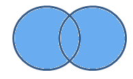
In simple words we can say that we should consider the probability of (A ꓴ B) when we are interested in combined probability of two (or more) events.
Intersection of Events
Let’s look at another example.
Let C be the event of getting a multiple of 2 and 3 when you throw a fair die.
Event A = Getting a multiple of 2 when you throw a fair die
Event B = Getting a multiple of 3 when you throw a fair die
Event C = Getting a multiple of 2 and 3
Event C is an intersection of event A & B.
Probabilities are then defined as follows.
P (C) = P (A ꓵ B)
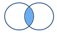
We can now say that the shaded region is the probability of both events A and B occurring together.
Disjoint Events
What if, you come across a case when any two particular events cannot occur at the same time.
For example: Let’s say you have a fair die and you have only one throw.
Event A = Getting a multiple of 3
Event B = Getting a multiple of 5
You want both event A & B should occur together.
Let’s find the sub space for Event A & B.
Event A = {3,6}
Event B = {5}
Sample Space= {1,2,3,4,5,6}
As you can see, there is no case for which event A & B can occur together. Such events are called disjoint event. To represent this using a Venn diagram:

Now that we are familiar with the terms Union, intersection and disjoint events, we can talk about independence of events.
90+ Python Interview Questions
Independent, Dependent & Exclusive Events
Suppose we have two events – event A and event B.
If the occurrence of event A doesn’t affect the occurrence of event B, these events are called independent events.
Let’s see some examples of independent events.
- Getting heads after tossing a coin AND getting a 5 on a throw of a fair die.
- Choosing a marble from a jar AND getting heads after tossing a coin.
- Choosing a 3 card from a deck of cards, replacing it, AND then choosing an ace as the second card.
- Rolling a 4 on a fair die, AND then rolling a 1 on a second roll of the die.
In each of these cases the probability of outcome of the second event is not affected at all by the outcome of the first event.
Probability of independent events
In this case the probability of P (A ꓵ B) = P (A) * P (B)
Let’s take an example here. Suppose we win the game if we pick a red marble from a jar containing 4 red and 3 black marbles and we get heads on the toss of a coin. What is the probability of winning?
Let’s define event A, as getting red marble from the jar
Event B is getting heads on the toss of a coin.
We need to find the probability of both getting a red marble and a heads in a coin toss.
P (A) = 4/7
P (B) = 1/2
We know that there is no affect of the color of the marble on the outcome of the coin toss.
P (A ꓵ B) = P (A) * P (B)
P (A ꓵ B) = (4/7) * (1/2) = (2/7)
Now, it’s time to implement the independent tests in R
Let us consider the following example:
Example:
We have two cards on which numbers are written on both front and back (1 at front and 2 at back). We will toss those two cards in air and see if the results of the two cards are independent. We toss the cards 2000 times, and then compute the joint distribution of the results of the toss from the two cards.
f <- function(toss=1){
  x <- sample(1:2, size=toss, replace=TRUE)
  y <- sample(1:2, size=toss, replace=TRUE)
  return(cbind(x,y))
}
set.seed(2500)
toss_times <- as.data.frame(f(2000))

library(plyr)

freq <- ddply(toss_times, ~x, summarize,
                    y1=sum(y==1), y2=sum(y==2))
row.names(freq) <- paste0('x',1:2)
prob_table1 <- freq_table[,-1]/2000
prob_table1


prob_x <- table(toss_times$x)/2000
prob_y <- table(toss_times$y)/2000
prob_table2 <- outer(prob_x,prob_y,'*')
row.names(prob_table2) <- paste0('x',1:2)
colnames(prob_table2) <- paste0('y',1:2)
prob_table2
Output
prob_table1
y1 y2
x1 0.2555 0.244
x2 0.2515 0.249

prob_table2

y1 y2
x1 0.2550247 0.2504752
x2 0.2494752 0.2450247
We see that prob_table1 and prob_table2 have close values, indicating that the toss of the two cards are probably independent.
Probability of dependent events
Next, can you think of examples of dependent events ?
In the above example, let’s define event A as getting a Red marble from the jar. We then keep the marble out and then take another marble from the jar.
Will the probabilities in the second case still be the same as that in the first case?
Let’s see. So, for the first time there are 4/7 chances of getting a red marble. Let’s assume you got a red marble on the first attempt. Now, for second chance, to get a red marble we have 3/6 chances.
If we didn’t get a red marble on the first attempt but a white marble instead. Then, there were 4/6 chances to get the red marble second time. Therefore the probability in the second case was dependent on what happened the first time.
Quiz 1: If you have a Jack and your next card is dealt with a new deck of cards the probability of you obtaining a jack again is? Are these events dependent or independent?
Mutually exclusive and Exhaustive events
Mutually exclusive events are those events where two events cannot happen together.
The easiest example to understand this is the toss of a coin. Getting a head and a tail are mutually exclusive because we can either get heads or tails but never both at the same in a single coin toss.
A set of events is collectively exhaustive when the set should contain all the possible outcomes of the experiment. One of the events from the list must occur for sure when the experiment is performed.
For example, in a throw of a die, {1,2,3,4,5,6} is an exhaustive collection because, it encompasses the entire range of the possible outcomes.
Consider the outcomes “even” (2,4 or 6) and “not-6” (1,2,3,4, or 5) in a throw of a fair die. They are collectively exhaustive but not mutually exclusive.
Quiz 2: Check whether the below events are mutually exclusive:
- Drawing a red card or a jack from a given 52 cards deck.
- Getting three heads or three tails when three coins are flipped.
Conditional Probability in R
Conditional probabilities in R arise naturally in the investigation of experiments where an outcome of a trial may affect the outcomes of the subsequent trials.
We try to calculate the probability of the second event (event B) given that the first event (event A) has already happened. If the probability of the event changes when we take the first event into consideration, we can safely say that the probability of event B is dependent of the occurrence of event A.
Let’s think of cases where this happens:
- Drawing a second ace from a deck given we got the first ace
- Finding the probability of having a disease given you were tested positive
- Finding the probability of liking Harry Potter given we know the person likes fiction
Here we can define, 2 events:
- Event A is the probability of the event we’re trying to calculate.
- Event B is the condition that we know or the event that has happened.
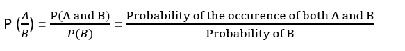
We can write the conditional probability in R as  , the probability of the occurrence of event A given that B has already happened.
Let’s Play a Simple Game of Cards For You to Understand This
Suppose you draw two cards from a deck and you win if you get a jack followed by an ace (without replacement). What is the probability of winning, given we know that you got a jack in the first turn?
Let event A be getting a jack in the first turn
Let event B be getting an ace in the second turn.
We need to find 
P(A) = 4/52
P(B) = 4/51 {no replacement}
P(A and B) = 4/52*4/51= 0.006
Here we are determining the probabilities when we know some conditions instead of calculating random probabilities. Here we knew that he got a jack in the first turn.
Let’s take another example.
Suppose you have a jar containing 6 marbles – 3 black and 3 white. What is the probability of getting a black given the first one was black too.
P (A) = getting a black marble in the first turn
P (B) = getting a black marble in the second turn
P (A) = 3/6
P (B) = 2/5
P (A and B) = ½*2/5 = 1/5
Let us now consider a new example and implement in R.
Example:
A research group collected the yearly data of road accidents with respect to the conditions of
following and not following the traffic rules of an accident prone area. They are interested in calculating the probability of accident given that a person followed the traffic rules. The table of the data is given as follows:
| Condition | Follow Traffic Rule | Does not follow Traffic Rule |
| Accident | 50 | 500 |
| No Accident | 2000 | 5000 |
Now here our equation becomes:
P(Accident | A person follow Traffic Rule) = P(Accident and follow Traffic Rule) / P(Follow Traffic Rule)
Solution:
P_Accident_who_follow_Traffic_Rule<-50

P_who_follow_Traffic_Rule=50+2000

Conditional_Probability=(P_Accident_who_follow_Traffic_Rule/P_who_follow_Traffic_Rule)
Conditional_Probability
Output
Conditional_Probability
0.02439024
Reversing the condition
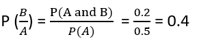
Example: Rahul’s favorite breakfast is bagels and his favorite lunch is pizza. The probability of Rahul having bagels for breakfast is 0.6. The probability of him having pizza for lunch is 0.5. The probability of him, having a bagel for breakfast given that he eats a pizza for lunch is 0.7.
Let’s define event A as Rahul having a bagel for breakfast, Event B as Rahul having a pizza for lunch.
P (A) = 0.6
P (B) = 0.5
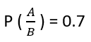
If we look at the numbers, the probability of having a bagel is different than the probability of having a bagel given he has a pizza for lunch. This means that the probability of having a bagel is dependent on having a pizza for lunch.
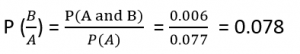
Now what if we need to know the probability of having a pizza given you had a bagel for breakfast. i.e. we need to know . Bayes theorem in R now comes into the picture.
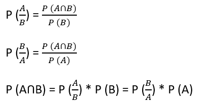
Bayes Theorem in R
The Bayes theorem in R describes the probability of an event based on the prior knowledge of the conditions that might be related to the event. If we know the conditional probability in R , we can use the bayes rule to find out the reverse probabilities .
How can we do that?
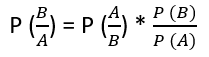
The above statement is the general representation of the Bayes rule.
For the previous example – if we now wish to calculate the probability of having a pizza for lunch provided you had a bagel for breakfast would be = 0.7 * 0.5/0.6.
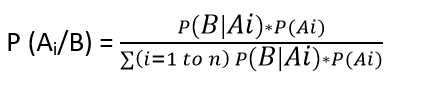
We can generalize the formula further.
If multiple events Ai form an exhaustive set with another event B.
We can write the equation as
Now, implementing the example in R:
#Bayes Theorem
cancer <- sample(c('No','Yes'), size=1000, replace=TRUE, prob=c(0.99852,0.00148))
test <- rep(NA, 1000) # creating a dummy variable
test[cancer=='No'] <- sample(c('Negative','Positive'), size=sum(cancer=='No'), replace=TRUE, prob=c(0.99,0.01))
test[cancer=='Yes'] <- sample(c('Negative','Positive'), size=sum(cancer=='Yes'), replace=TRUE, prob=c(0.07, 0.93))


P_cancer_and_pos<-0.00148*0.93
P_no_cancer_and_pos<-0.99852*0.01

Bayes_Theorem<-(P_cancer_and_pos/(P_cancer_and_pos+P_no_cancer_and_pos))
Bayes_Theorem
Output
Bayes_Theorem
0.1211449
Example of Bayes Theorem in R and Probability trees
Let’s take the example of the breast cancer patients. The patients were tested thrice before the oncologist concluded that they had cancer. The general belief is that 1.48 out of a 1000 people have breast cancer in the US at that particular time when this test was conducted. The patients were tested over multiple tests. Three sets of test were done and the patient was only diagnosed with cancer if she tested positive in all three of them.
Examine the Test in Details
Sensitivity of the test (93%) – true positive Rate
Specificity of the test (99%) – true negative Rate
Let’s first compute the probability of having cancer given that the patient tested positive in the first test.
P (has cancer | first test +)
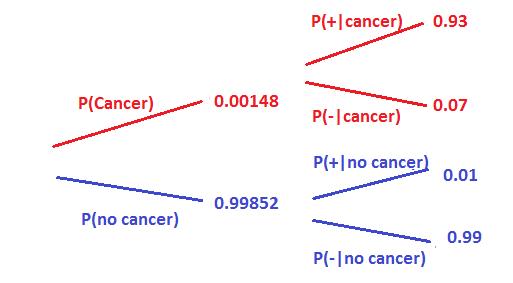
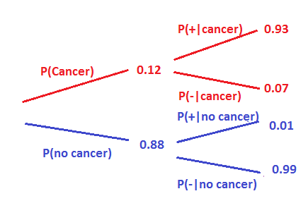
P (cancer) = 0.00148
Sensitivity can be denoted as P (+ | cancer) = 0.93
Specificity can be denoted as P (- | no cancer)
Since we do not have any other information, we believe that the patient is a randomly sampled individual. Hence our prior belief is that there is a 0.148% probability of the patient having cancer.
The complement is that there is a 100 – 0.148% chance that the patient does not have CANCER. Similarly we can draw the below tree to denote the probabilities.
Let’s now try to calculate the probability of having cancer given that he tested positive on the first test i.e. P (cancer|+)
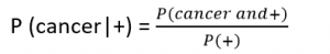
P (cancer and +) = P (cancer) * P (+) = 0.00148*0.93
P (no cancer and +) = P (no cancer) * P(+) = 0.99852*0.01
To calculate the probability of testing positive, the person can have cancer and test positive or he may not have cancer and still test positive.
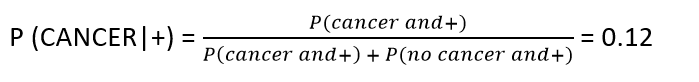
This means that there is a 12% chance that the patient has cancer given he tested positive in the first test. This is known as the posterior probability.
Bayes Updating
Let’s now try to calculate the probability in bayes theorem in R of having cancer given the patient tested positive in the second test as well.
Now remember bayes theorem in R we will only do the second test if she tested positive in the first one. Therefore now the person is no longer a randomly sampled person but a specific case. We know something about her. Hence, the prior probabilities should change. We update the prior probability with the posterior from the previous test.
Nothing would change in the sensitivity and specificity of the test since we’re doing the same test again. Look at the bayes theorem in R probability tree below.
Let’s calculate again the probability of having cancer given she tested positive in the second test.
P (cancer and +) = P(cancer) * P(+) = 0.12 * 0.93
P (no cancer and +) = P (no cancer) * P (+) = 0.88 * 0.01
To calculate the probability of testing positive, the person can have cancer and test positive or she may not have cancer and still test positive.

Now we see, that a patient who tested positive in the test twice, has a 93% chance of having cancer.
Frequentist vs Bayesian Definitions of probability
A frequentist defines probability as an expected frequency of occurrence over large number of experiments.
P(event) = n/N, where n is the number of times event A occurs in N opportunities.
The Bayesian view of probability is related to degree of belief. It is a measure of the plausibility of an event given incomplete knowledge.
The frequentist believes that the population mean is real but unknowable and can only be estimated from the data. He knows the distribution of the sample mean and constructs a confidence interval centered at the sample mean. So the actual population mean is either in the confidence interval or not in it.
This is because he believes that the true mean is a single fixed value and does not have a distribution. So the frequentist says that 95% of similar intervals would contain the true mean, if each interval were constructed from a different random sample.
The Bayesian definition has a totally different view point. They use their beliefs to construct probabilities. They believe that certain values are more believable than others based on the data and our prior knowledge.
The Bayesian constructs a credible interval centered near the sample mean and totally affected by the prior beliefs about the mean. The Bayesian can therefore make statements about the population mean by using the probabilities.
Open Challenges
- In the cancer example taken above, try calculating the probability of a patient having cancer provided the patient is tested positive in the third test as well.
- In an exam, there is a problem that 60% of students know the correct answer. However, there is 15% chance that a student picked the wrong answer even if he/she knows the right answer And there is also a 25% chance that a student does not know the right answer but guessed it correctly. If a student did get the problem right, what is the chance that this student really knows the answer?
Conclusion
A solid grasp of probability is indispensable for data science practitioners, as many data science problems are inherently probabilistic. Conditional probability in R plays a crucial role in understanding and implementing algorithms effectively. Through this article, we delved into various concepts, from basic terminologies like union, intersection, and disjoint events to more advanced topics like conditional probability and Bayes’ Theorem in R. By providing real-world examples and practical implementations, we aimed to enhance your comprehension of these concepts. Embracing both frequentist and Bayesian perspectives, we navigated through challenges and questions, empowering you with valuable insights into probabilistic thinking essential for data science endeavors.
Frequently Asked Questions
A. Conditional probability in R calculates the likelihood of an event given another event has occurred. Bayes’ Theorem, an extension, incorporates prior probabilities to compute the probability of a cause/event based on the observed effect. It’s used to update beliefs as new information arises. Bayes’ Theorem provides a structured way to adjust probabilities using prior knowledge, making it fundamental in various fields like statistics and machine learning.
A. Bayes’ Theorem in R is a formula that calculates the probability of an event A occurring given that event B has occurred. It’s expressed as P(A|B) = (P(B|A) * P(A)) / P(B), where P(A) and P(B) are the probabilities of events A and B, and P(B|A) is the probability of event B given event A. It’s a cornerstone of probabilistic reasoning and inference.
A. Conditional probability in R calculates the likelihood of an event given another event has occurred, essential for probabilistic reasoning.
A. Bayes’ Theorem in R incorporates prior probabilities to compute the probability of a cause/event based on observed effects.
A. Probability is essential in data science as many problems are probabilistic, requiring algorithms and models based on probabilistic reasoning for effective analysis.
Dishashree is passionate about statistics and is a machine learning enthusiast. She has an experience of 1.5 years of Market Research using R, advanced Excel, Azure ML.


Nice article! One basic doubt ....prob of can cer and + is calculated as prob cancer * prob of positive = 0.00148*0.93....but we multiply probabilities only if they are independent events correct? Since prob of positive changes with without cancer these are dependent right
The probability of +ve given you have cancer is the true positive rate of the test, which is always fixed for the test. Here the positive means the probability of testing positive given you have cancer. If you check the value 0.93 it is P(+|cancer) and not just P(+).
Could you also post the answer to the quizzes and open challenges . That way , we can verify the answers which we have got with the correct answers
Open Challenges Answers: 1. 0.999162 2. 0.836066
On page 8 in the conditional probability section the first event B is the event that has already happened, but later in the page, its event A (getting a Jack), not B, that is the event that has already happened. Switching the letters is confusing. In addition, in the first part of the game the first draw is a jack, but later in the game it states "Here we knew that he got an ace in the first draw." Please clarify. Thank you.
Hey Edward, thanks for pointing that out, “Here we knew that he got an ace in the first draw" has been edited to "got a jack in the first draw". Small clarification, So the event which we know has happened is the condition that we already know for sure. In this case we knew that the first draw was a jack, hence that was the condition on which the further probability is based. If the letters confuse you, I would encourage solving these examples again with taking the known condition as B and always calculating P(A/B). Do post if you need further clarification!
1. 0.9980 2. 0.8360
I think this line is incorrect: P (no cancer and +) = P (no cancer) * P(+) = 0.99852*0.99 The correct statement should be --- 0.998582 * 0.01 12 % though is correct & is based on the 2nd formula which I mentioned.
this has been corrected.. Thanks !
Nice work!
A well written and a very informative article for the aspiring data science professionals.. Keep up the good work !
1: 0,93 x 0,9276 / (0,93 x 0,9276 + 0,0724 x 0,01) = 0,9942 2: 0,85 x 0,6 / (0,85 x 0,6 + 0,25 x 0,4) = 0,8361
It's interesting that many of the bloggers to helped clarify a few things for me as well as giving.Most of ideas can be nice content.The people to give them a good shake to get your point and across the command.
An excellent article for budding data science professionals to get their basics right. Looking forward to more such articles!
1. 0.99 2. o.83
Well written and thanks for the article. I would need a clarification here. How can we consider P(Cancer)=0.12 for the second test. Here, 12% is a chance that the patient has cancer given he tested positive and it's not the probability of having the cancer. Could please help me to understand here
Nice Article. I learned a lot Piush Vaish http://adataanalyst.com/
Great article and well said. Quick correction at "Let’s NOT try to calculate the probability of having cancer given that he tested positive on the first test i.e. P (cancer|+)" There shouldn't be NOT in above statement.
agreed; perhaps a simple typo - "let's NOW try ..."
Nice article I am a school teacher, I learn a lot from ur article it help me to explain the students with example. Thanks
Top stuff, Was really helpful in refreshing the probability concepts and the rationale behind Bayes. Thanks
Nice Article !!
Thank you!
Statistics and probability is my favorite course please share your material as much as possible.