Statistics for Data Science: What is Normal Distribution?
Introduction to the Normal Distribution
Have you heard of the bell curve? It tends to be among the most discussed water-cooler topics among people around the globe. For a long time, a bell curve dictated the professional assessment of an employee and was a beloved or dreaded topic, depending on who to spoke to!
Take a look at this image:
 Source: empxtrack.com
What do you think the shape of the curve signifies? As a data scientist (or an aspiring one), you should be able to answer that question at the drop of a hat. The idea behind a bell curve, among many other applications, is that of a normal distribution.
The normal distribution is a core concept in statistics, the backbone of data science. While performing exploratory data analysis, we first explore the data and aim to find its probability distribution, right? And guess what – the most common probability distribution is Normal Distribution.
Check out these three very common examples of the normal distribution:
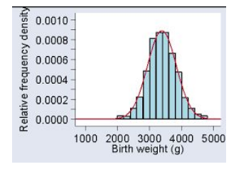
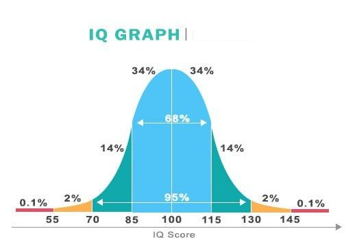
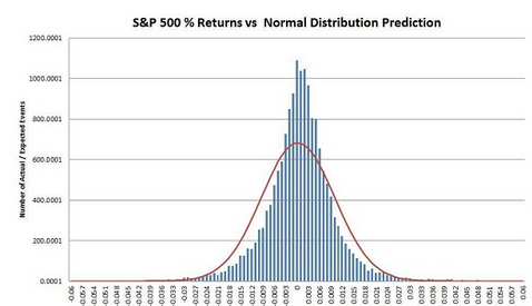
As you can clearly see, the Birth weight, the IQ Score, and stock price return often form a bell-shaped curve. Similarly, there are many other social and natural datasets that follow Normal Distribution.
One more reason why Normal Distribution becomes essential for data scientists is the Central Limit Theorem. This theorem explains the magic of mathematics and is the foundation for hypothesis testing techniques.
In this article, we will be understanding the significance and different properties of Normal Distribution and how we can use those properties to check the Normality of our data.
Table of Contents
- Properties of Normal Distribution
- Empirical Rule for Normal Distribution
- What is a Standard Normal Distribution?
- Getting Familiar with Skewed Distribution
- Left Skewed Distribution
- Right Skewed Distribution
- How to check the Normality of a Distribution
-
- Histogram
- KDE Plots
- Q_Q Plots
- Skewness
- Kurtosis
-
- Python Code to Implement and Understand Normal Distribution
Properties of Normal Distribution


We call this Bell-shaped curve a Normal Distribution. Carl Friedrich Gauss discovered it so sometimes we also call it a Gaussian Distribution as well.
We can simplify the Normal Distribution’s Probability Density by using only two parameters: 𝝻 Mean and 𝛔2. This curve is symmetric around the Mean. Also as you can see for this distribution, the Mean, Median, and Mode are all the same.
One more important phenomena of a normal distribution is that it retains the normal shape throughout, unlike other probability distributions that change their properties after a transformation. For a Normal Distribution:
- Product of two Normal Distribution results into a Normal Distribution
- The Sum of two Normal Distributions is a Normal Distribution
- Convolution of two Normal Distribution is also a Normal Distribution
- Fourier Transformation of a Normal Distribution is also Normal
Starting to realize the power of this incredible concept?
Empirical Rule for Normal Distribution
Have you heard of the empirical rule? It’s a commonly used concept in statistics (and in a lot of performance reviews as well):
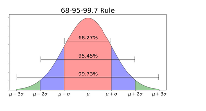
According to the Empirical Rule for Normal Distribution:
- 68.27% of data lies within 1 standard deviation of the mean
- 95.45% of data lies within 2 standard deviations of the mean
- 99.73% of data lies within 3 standard deviations of the mean
Thus, almost all the data lies within 3 standard deviations. This rule enables us to check for Outliers and is very helpful when determining the normality of any distribution.
What is a Standard Normal Distribution?
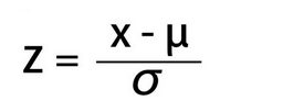
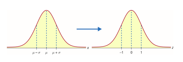
Standard Normal Distribution is a special case of Normal Distribution when 𝜇 = 0 and 𝜎 = 1. For any Normal distribution, we can convert it into Standard Normal distribution using the formula:
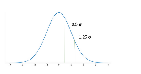
To understand the importance of converting Normal Distribution into Standard Normal Distribution, let’s suppose there are two students: Ross and Rachel. Ross scored 65 in the exam of paleontology and Rachel scored 80 in the fashion designing exam.
Can we conclude that Rachel scored better than Ross?
No, because the way people performed in paleontology may be different from the way people performed in fashion designing. The variability may not be the same here.
So, a direct comparison by just looking at the scores will not work.
Now, let’s say the paleontology marks follow a normal distribution with mean 60 and a standard deviation of 4. On the other hand, the fashion designing marks follow a normal distribution with mean 79 and standard deviation of 2.
We will have to calculate the z score by standardization of both these distributions:
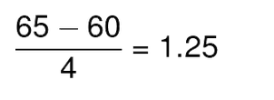
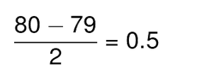
Thus, Ross scored 1.25 standard deviations above the mean score while Rachel scored only 0.5 standard deviations above the mean score. Hence we can say that Ross Performed better than Rachel.
Let’s Talk About the Skewed Distribution
Normal Distribution is symmetric, which means its tails on one side are the mirror image of the other side. But this is not the case with most datasets. Generally, data points cluster on one side more than the other. We call these types of distributions Skewed Distributions.
Left Skewed Distribution
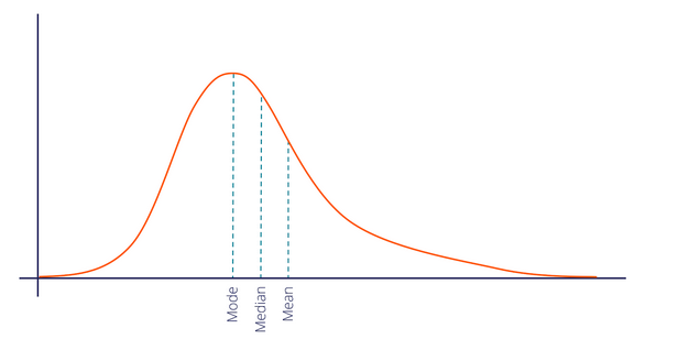
When data points cluster on the right side of the distribution, then the tail would be longer on the left side. This is the property of Left Skewed Distribution. The tail is longer in the negative direction so we also call it Negatively Skewed Distribution.
 Here, Mode > Median > Mean.
In the Normal Distribution, Mean, Median and Mode are equal but in a negatively skewed distribution, we express the general relationship between the central tendency measured as:
Mode > Median > Mean
Right Skewed Distribution
When data points cluster on the left side of the distribution, then the tail would be longer on the right side. This is the property of Right Skewed Distribution. Here, the tail is longer in the positive direction so we also call it Positively Skewed Distribution.
In a positively skewed distribution, we express the general relationship between the central tendency measures as:
Mode < Median < Mean
How to Check the Normality of a Distribution
The big question! To check the normality of data, let’s take an example where we have the information of the marks of 1000 students for Mathematics, English, and History. You can find the Dataset here.
You can find the code in the later section of this article.
Let’s see a few different ways to check the normality of the distribution that we have.
Histogram
- A Histogram visualizes the distribution of data over a continuous interval
- Each bar in a histogram represents the tabulated frequency at each interval/bin
- In simple words, height represents the frequency for the respective bin (interval)
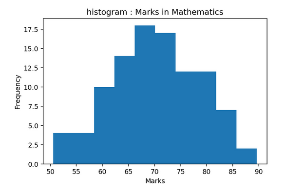
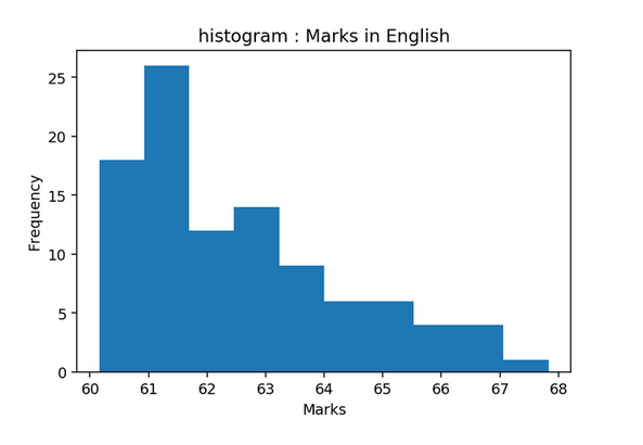
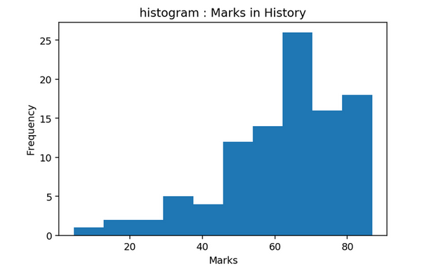
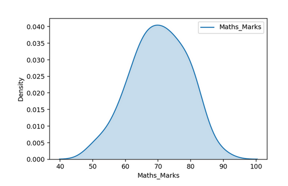
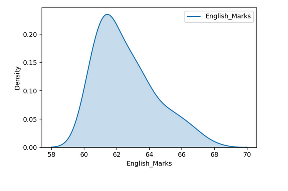
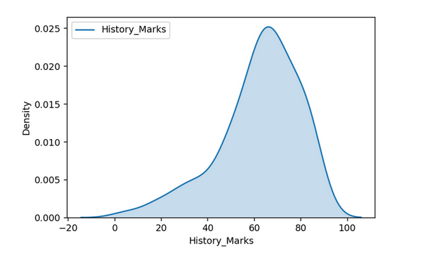
As you can see here, Mathematics follows the Normal Distribution, English follows the right-skewed distribution and History follows the left-skewed distribution.
KDE Plots
Histogram results can vary wildly if you set different numbers of bins or simply change the start and end values of a bin. To overcome this, we can make use of the density function.
A density plot is a smoothed, continuous version of a histogram estimated from the data. The most common form of estimation is known as kernel density estimation (KDE). In this method, a continuous curve (the kernel) is drawn at every individual data point and all of these curves are then added together to make a single smooth density estimation.
Q_Q Plot
Quantiles are cut points dividing the range of a probability distribution into continuous intervals with equal probabilities or dividing the observations in a sample in the same way.
- 2 quantile is known as the Median
- 4 quantile is known as the Quartile
- 10 quantile is known as the Decile
- 100 quantile is known as the Percentile
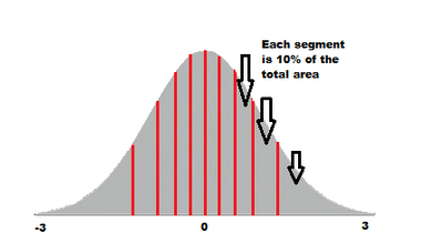
10 quantile will divide the Normal Distribution into 10 parts each having 10 % of the data points. The Q-Q plot or quantile-quantile plot is a scatter plot created by plotting two sets of quantiles against one another.
Here, we will plot theoretical normal distribution quantiles and compare them against observed data quantiles: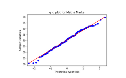
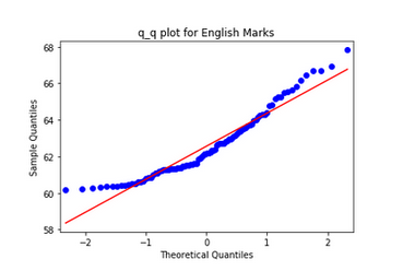
For Mathematics Marks, values follow the straight line indicating that they come from a Normal Distribution. On the other side for English Marks, larger values are larger as expected from a Normal Distribution and smaller values are not as small as expected from a Normal Distribution which is also the case in a right-skewed distribution.
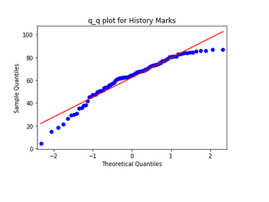
While for History Marks, larger values are not as large as expected from a Normal Distribution and smaller values are smaller as expected from a Normal Distribution which happens to be the case in a left-skewed distribution.
The Concept of Skewness
Skewness is also another measure to check for normality which tells us the amount and direction of the skewed data points. Generally for the value of Skewness:
- If the value is less than -0.5, we consider the distribution to be negatively skewed or left-skewed where data points cluster on the right side and the tails are longer on the left side of the distribution
- Whereas if the value is greater than 0.5, we consider the distribution to be positively skewed or right-skewed where data points cluster on the left side and the tails are longer on the right side of the distribution
- And finally, if the value is between -0.5 and 0.5, we consider the distribution to be approximately symmetric
What is Kurtosis?
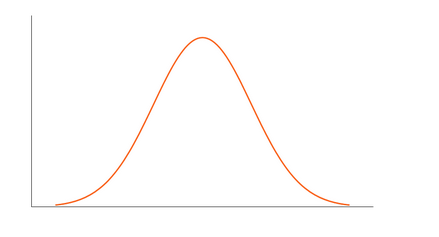
Another numerical measure to check for Normality is Kurtosis. Kurtosis gives the information regarding tailedness which basically indicates the data distribution along the tails.
For the symmetric type of distribution, the Kurtosis value will be close to Zero. We call such types of distributions as Mesokurtic distribution. Its tails are similar to Gaussian Distribution.
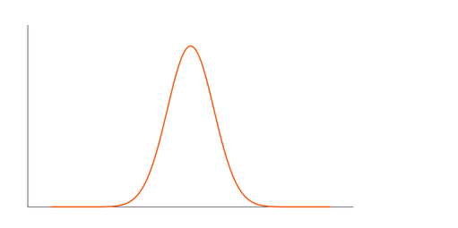
If there are extreme values present in the data, then it means that more data points will lie along with the tails. In such cases, the value of K will be greater than zero. Here, Tail will be fatter and will have longer distribution. We call such types of distributions as Leptokurtic Distribution. As we can clearly see here, the tails are fatter and denser as compared to Gaussian Distribution:
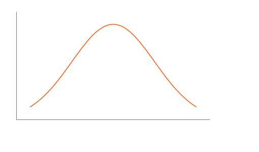
If there is a low presence of extreme values compared to Normal Distribution, then lesser data points will lie along the tail. In such cases, the Kurtosis value will be less than zero. We call such types of distributions as Platykurtic Distribution. It will have a thinner tail and a shorter distribution in comparison to Normal distribution.
Python Code to Understand Normal Distribution
Here’s the full Python code to implement and understand how a normal distribution works.
import numpy as np
import pandas as pd
import seaborn as sns
import matplotlib.pyplot as plt
import statsmodels.api as sm
df = pd.read_csv('Marks.csv')
def UVA_numeric(data):
    var_group = data.columns
    size = len(var_group)
    plt.figure(figsize = (7*size,3), dpi = 400)

    #looping for each variable
    for j,i in enumerate(var_group):


        # calculating descriptives of variable
        mini = data[i].min()
        maxi = data[i].max()
        ran = data[i].max()-data[i].min()
        mean = data[i].mean()
        median = data[i].median()
        st_dev = data[i].std()
        skew = data[i].skew()
        kurt = data[i].kurtosis()

        # calculating points of standard deviation
        points = mean-st_dev, mean+st_dev

        #Plotting the variable with every information
        plt.subplot(1,size,j+1)
        sns.distplot(data[i],hist=True, kde=True)

        sns.lineplot(points, [0,0], color = 'black', label = "std_dev")
        sns.scatterplot([mini,maxi], [0,0], color = 'orange', label = "min/max")
        sns.scatterplot([mean], [0], color = 'red', label = "mean")
        sns.scatterplot([median], [0], color = 'blue', label = "median")
        plt.xlabel('{}'.format(i), fontsize = 20)
        plt.ylabel('density')
        plt.title('std_dev = {}; kurtosis = {};\nskew = {}; range = {}\nmean = {}; median = {}'.format((round(points[0],2),round(points[1],2)),
                                                                                                       round(kurt,2),
                                                                                                       round(skew,2),
                                                                                                       (round(mini,2),round(maxi,2),round(ran,2)),
                                                                                                       round(mean,2),
                                                                                                       round(median,2)))
UVA_numeric(df)

End Notes
In this article, we followed a step by step procedure to understand the fundamentals of Normal Distribution. We also understood the concepts of determining the Normality, like Histogram, KDE, Q_Q Plot, Skewness, and Kurtosis.
For more details about statistical concepts, you can also read these articles:
- 6 Common Probability Distributions every data science professional should know
- Introduction to Central Limit Theorem
Did you find this article useful? Can you think of any other distributions similar to Normal distribution like F-distributions, Chi-Square distribution or t-distribution, and their applications? Let me know in the comments section below and we can come up with more ideas to explore them.


Informative one... Looking forward for more such contents.
Outstanding Blog