Getting into Random Forest Algorithms

Nibin Vidhyadharan 30 Apr, 2021 • 8 min read

This article was published as a part of the Data Science Blogathon.

Before I get into explaining the random forest algorithms and how to work with them, there are some other basic we need to understand the first concept is the

Ensemble learning
Bagging
Decision trees

Ensemble learning

Ensemble learning is an ML paradigm where numerous base models (which are often referred to as “weak learners”) are combined and trained to solve the same problem. This method is based on the theory that by correctly combining several base models together, these weak learners can be used as building blocks for designing more complex ML models.

The simplest way to think about ensemble learning is something called the wisdom of the crowd. There is an interesting experiment of predicting the number of chocolates in a jar, the experimenter introduces a jar full of chocolate to a crowd and asks them to predict it. Everyone in the crowd come up with their own prediction, on the number of chocolates in the jar. When the experimenter added all the predictions and took the average of it their number was very approximate to the actual prediction. This experiment was conducted several times and record a very similar outcome.

Ensemble learning also works very similarly to that. Here were are going to stack up several weak learners to make a very approximate prediction. There are a set of algorithms under this very same idea that uses different types of weak learners to make robust and sometimes complex machine learning models. The core idea of using a sequence of weak learners remains the same, all of them vary in how they are implemented. A lot of them are very near to tree-based machine learning models.

Before we get into understanding the random forest algorithm there are some of the basics we need to understand,

Decision trees
Bagging

Decision trees

Here we are not going to get to details into the nitty-gritty of the decision tree, we will talk discuss that in a later blog.
The simple decision, tress is a machine learning model, where we make predictions through a tree-based model. In simple, a decision tree asks a sequence of questions on the input data and each of the answers gives the tree a direction to predict the results.

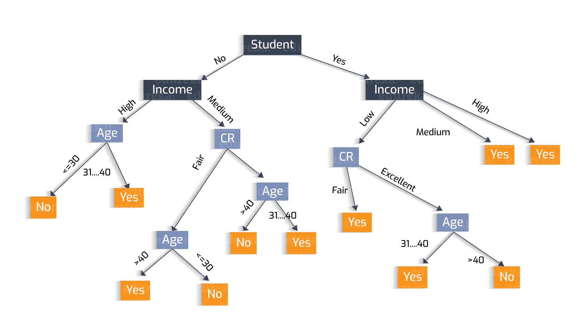
These are some image to give you a context of how a decision tree looks like, there are several paraments to this, from

How does the decision tree choose features to split the tree?
How does the splitting happen?
What are some disadvantages of these trees?
How does the decision tree work in the case of regression problems?
How reliable is this prediction?

Out of all these questions we are going to pick the last question How reliable is this prediction?

How reliable is decision tree prediction?

In the domain of machine learning, we have this concept of bias and variance. The idea of any machine learning or deep learning algorithm is to generalize the phenomena through data inputs. The general assumption is that everything forms a pattern and this pattern are influenced by different features if we could figure out how this feature influences the pattern then we could predict phenomena. Almost all the machine learning models are looking into this pattern and try to generalize this pattern in different ways.

How do we determine the quality of a machine learning model?

The quality is determined by looking into something called variances and bias.

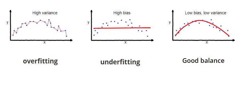
decision tree prediction algorithms random forest

As you can see from the image overfitting Is a scenario when your prediction fits exactly on top of the input/testing data. This is considered a corrupt machine learning model since the idea of the model is not to fit on top of the input data but rather to understand the pattern of the data (as seen in good balance). This entire overfitting completely ignores the overall big picture of the data.

There is another case that tries to understand the overall picture of the data and still fails this is called high bias. In this scenario, your model is not sticking to the input data but is trying to generalize the overall pattern of the model again it’s not good enough to do the job.

What is an ideal model?

So ideally we are looking at a model that gives us low bias and low variance. (third image). For any machine learning model, this is a standard method to estimate. How well this model is performing. When you create training data we split the data into 2 parts, training and testing, The training data train the machine learning model and the testing data is used to test how well the model is performing in the model.

There are cases when you train the model you get fewer errors and when you test the data the error rate explodes this is because your model just over-fitted while training. When you have high biases your model performs terribly with pretty much high error values while training itself. Partly because the predictions are far away from the real values.

What is the disadvantage of a decision tree?

One of the biggest disadvantages of the decision tree is, it tends to overfit data. It means we could see the data trained with the decision tree tended to show high variance and creates false predictions in the test data.

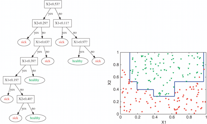
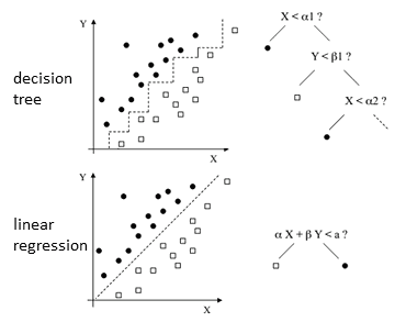
disadvantage of a decision tree random algorithms

It’s not necessary that decision trees over fit all the cases, why does this happen, a decision tree makes its prediction through asking a series of questions, for a visual context you can imagine a decision tree question(node) is trying a separate region where it can find the most suitable prediction. In linear regression,

a decision line is drawn in between two classifications. A decision tree asking a series of questions to draw a decision boundary. Diagrams of the decision tree and the linear regression explain how both of the algorithms make the decision. As you can see that the behavior of the decision tree itself is to approach the training data through the sequence of questions rather than understanding the general pattern of the data.

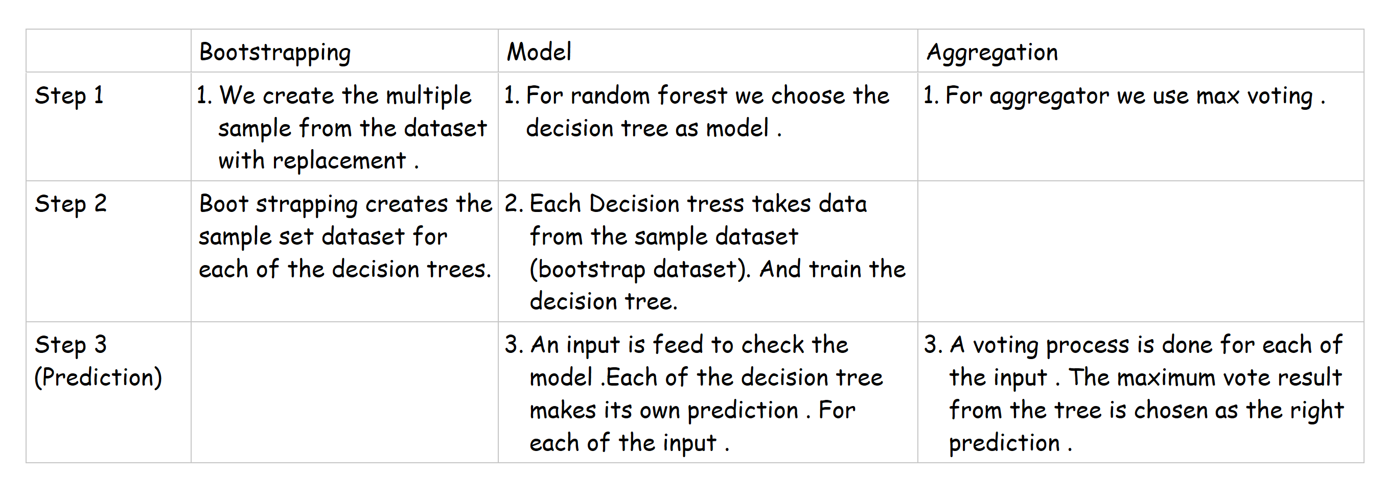
What are bootstrapping and bagging?

There is a little bit of confusion on terms like bagging, boost strapping, aggregation, pasting, replacement, etc. All these terminologies are closely related to the bagging itself lets put some clarity into this terminology and move further.

Bootstrapping :

Boost strapping is a process of creating a subset of data from the original data. There are several flavors of this

Pasting

When random subsets of the dataset are drawn as random subsets of the samples, then this algorithm is known as Pasting.

Bagging

When samples are drawn with replacement, then the method is known as Bagging. When you say replacement it means you are allowing the duplication of the data.

So Bagging is a sampling technique in which we create subsets of observations from the original dataset, with replacement. The size of the subsets is the same as the size of the original set.

Multiple subsets are created from the original dataset, selecting observations with replacement.
A base model (weak model) is created on each of these subsets.
The models run in parallel and are independent of each other.
The final predictions are determined by combining the predictions from all the models

Random Subspace

When random subsets of the dataset are drawn as random subsets of the features, then the method is known as Random Subspaces.

Random Patches

Finally, when base estimators are built on subsets of both samples and features, then the method is known as Random Patches.

Aggregation :

Model predictions undergo aggregation to combine them for the final prediction to consider all the outcomes possible. The aggregation can be done based on the total number of outcomes or on the probability, or using any traditional techniques like max voting, average voting, soft voting, weightage voting .of predictions derived from the bootstrapping of every model in the procedure.

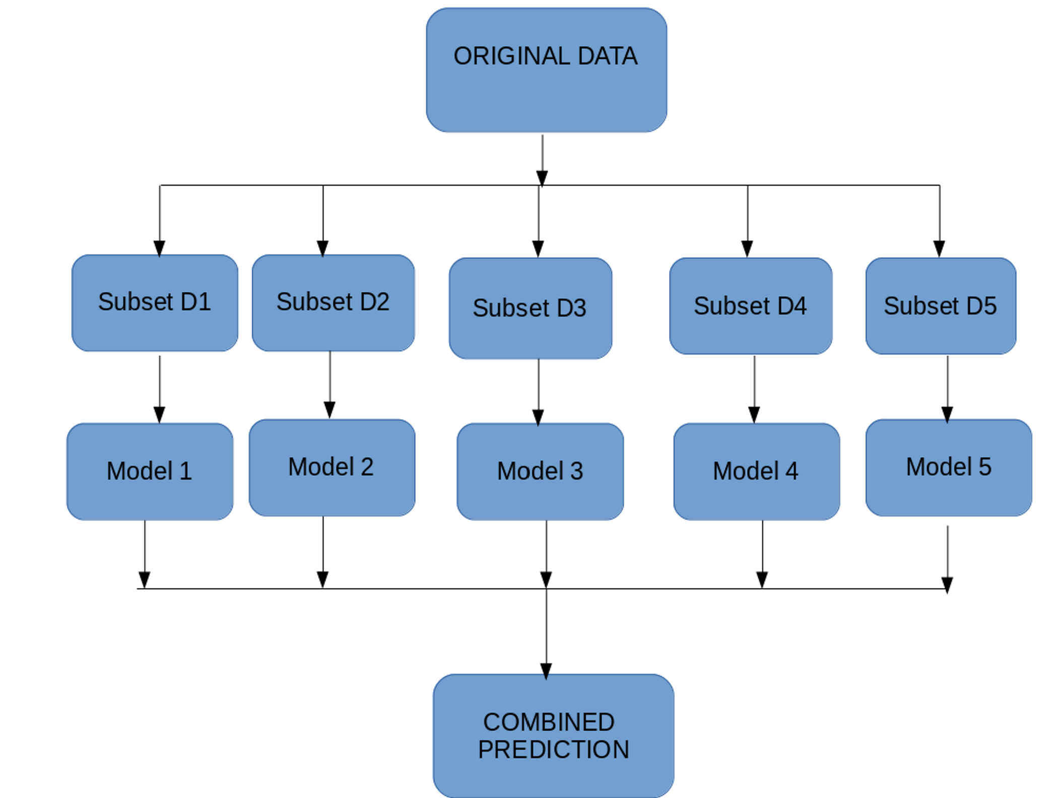
This is the basic structure of bagging, it starts with the original data, several subsets of the original data are created, this is run through several models, then an aggregator is used to make the prediction.

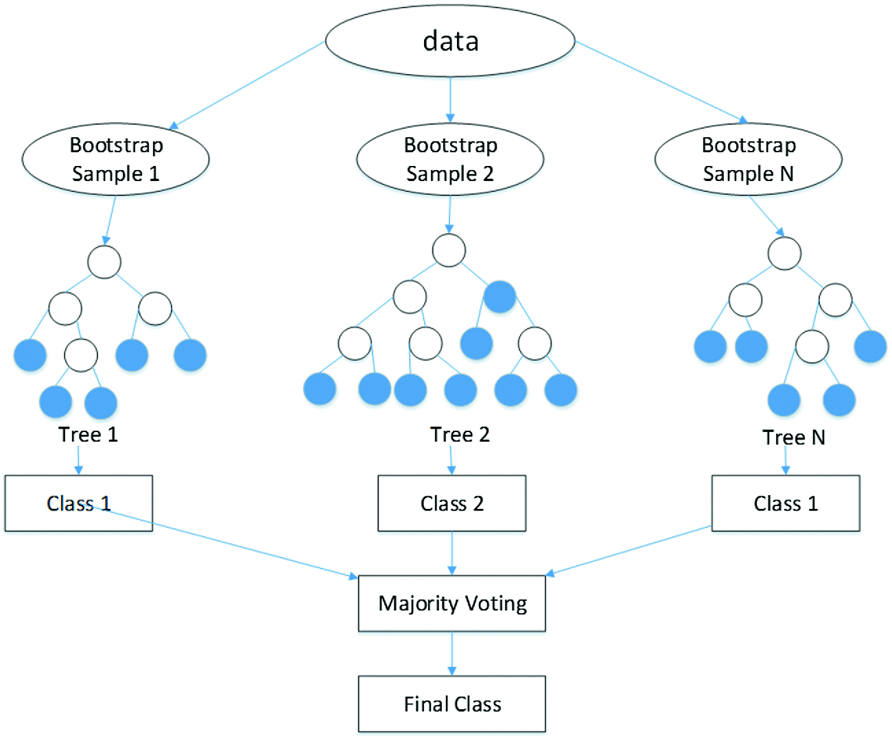
Random forest

A random forest is basically a combination of bagging with trees. You have the freedom to using any model in bagging, when you use a tree-based model then it’s called a random forest.

Proof of concept

This title is called the proof of the concept simply because I introduced the random forest as a usage of the bagging method in the decision tree. So we will first look into building the decision tree with the bagging ideas itself. We will progress to the most high-level approach we have in the sklearn that is the random forest object. Through which we can create a random forest easily.

from sklearn.ensemble import BaggingClassifier
from sklearn.tree import DecisionTreeClassifier

#creating the bagging classifer 
'''here we are going to create the bagging classifer and providing the tree as the estimatr'''
 
bag_clf = BaggingClassifier( DecisionTreeClassifier(),n_estimators=500,max_samples=100,
bootstrap=True,n_jobs=-1) 

bag_clf.fit(X_train, y_train) y_pred = bag_clf.predict(X_test)

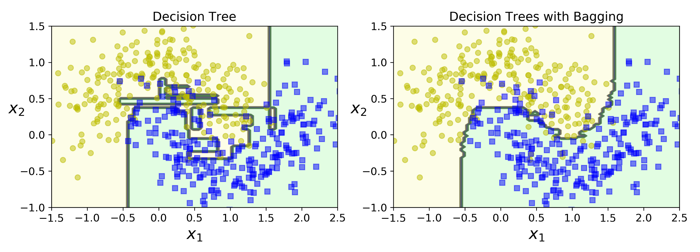
This is the code its a simple 5 line code we are simply implementing a bagging classifier, and inside we are going to apply a decision, tree-based estimator. In the above image, you can see that what does a bagging process does to the decision tree. It almost smoothened the decision boundary and provided a very smooth decision area. You can also observe that there is very little overfitting of the data compared to the classical decision tree itself.

Using the high-level implementation in sklearn

This is the high-level implementation of the random forest provided by sklearn. With this function, we can directly create the random forest without much effort.

from sklearn.datasets import load_iris
from sklearn.ensemble import RandomForestClassifier
iris = load_iris()
rnd_clf = RandomForestClassifier(n_estimators=500, n_jobs=-1) rnd_clf.fit(iris["data"], iris["target"])

for name, score in zip(iris["feature_names"],rnd_clf.feature_importances_):
    print(name, score)

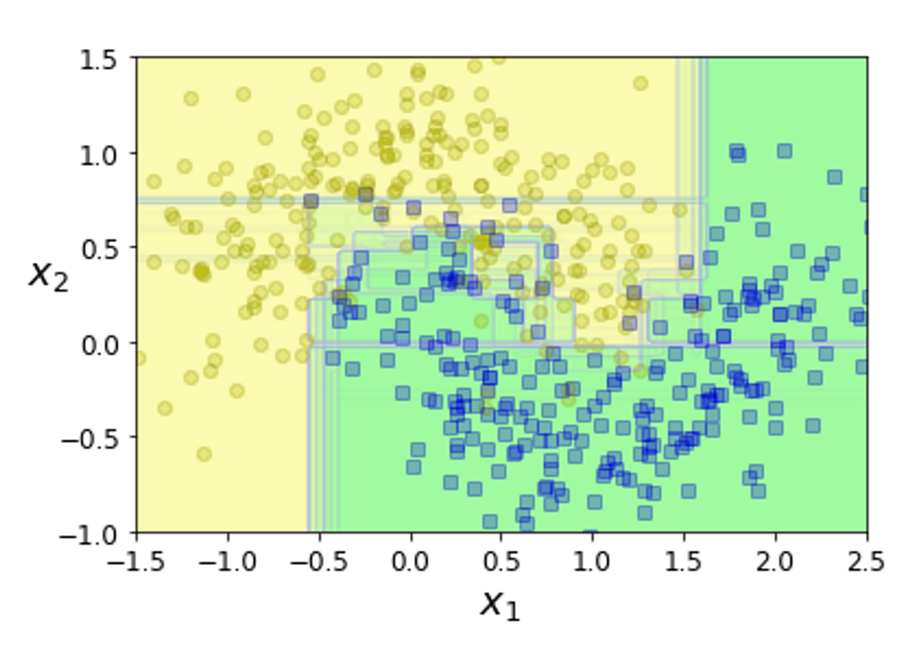
This is the high-level implementation of the random forest provided by sklearn. With this function, we can directly create the random forest without much effort.

This is what random forest does to the data. As you can see there are several boundary lines. Each of the boundary lines is drawn by each of the estimators.

How does the hyperparameter work?

Here am going to mention some of the very important parameters in the random forest, do check out the sklearn documentation attached below for more parameters.

Summary:

In layman terms

So this is what random forest all about, you create 1000+ (n_estimator) decision trees.
Take prediction from each of the decision trees.
They are combined together and a voting processing is done (aggregation), the maximum vote is chosen as the right prediction.

This is an explanation for the random forest for the classification problem, in the coming blogs we will look into the random forest for a regression problem, please do share this blog if you liked it, comment with your suggestions and questions, the blogs are constantly updated your reviews will be considered in the upcoming updates.

Reference

I do recommend you to check out the reference links, provided below for the clarity

Decision Tree Video (most recommended)

From <https://www.youtube.com/watch?v=7VeUPuFGJHk&t=736s >

Random Forest

From <https://www.youtube.com/watch?v=J4Wdy0Wc_xQ >

The media shown in this article on random forest algorithms are not owned by Analytics Vidhya and is used at the Author’s discretion.

blogathon Random Forest Algorithm

Nibin Vidhyadharan 30 Apr 2021

Beginner Classification Machine Learning Regression