Wine Quality Prediction Using Machine Learning
Overview
- Basics understanding of Wine.
- Data description
- Importing modules
- Study dataset
- Visualization
- Handle null values
- Split dataset
- Normalization
- Applying model
- Save model
- Endnote
Introduction
” Wine is the most healthful and most hygienic of beverages “
– Louis Pasteur
Yes, if you think deep down then you just notice that we are discussing wine, above quote seems to be right because all over the world wine was soo popular among people, and 5% of the population doesn’t know what is wine? sounds good.
We definitely came across the fruit graphs, which is soo sweet on the test but graphs are not just to eat, they are used to make different types of things. Wine is one of them Wine is an alcoholic drink that is made up of fermented grapes. If you have come across wine then you will notice that wine has also their type they are red and white wine this was because of different varieties of graphs.
You are shocked to hear that the worldwide distribution of wine is 31 million tonnes which were huge in number.
What if you think about the quality of wine, how can you differentiate the wine according to their quality? The big question arises.
According to experts, the wine is differentiated according to its smell, flavor, and color, but we are not a wine expert to say that wine is good or bad. What will we do then? Here’s the use of Machine Learning comes, yes you are thinking to write we are using machine learning to check wine quality. ML have some techniques that will discuss below:
To the ML model, we first need to have data for that you don’t need to go anywhere just click here for the wine quality dataset. This dataset was picked up from the Kaggle.
Now, we start our journey towards the prediction of wine quality, as you can see in the data that there is red and white wine, and some other features. Let’s start :
Description of Dataset
If you download the dataset, you can see that several features will be used to classify the quality of wine, many of them are chemical, so we need to have a basic understanding of such chemicals.
- volatile acidity : Volatile acidity is the gaseous acids present in wine.
- fixed acidity : Primary fixed acids found in wine are tartaric, succinic, citric, and malic
- residual sugar : Amount of sugar left after fermentation.
- citric acid : It is weak organic acid, found in citrus fruits naturally.
- chlorides : Amount of salt present in wine.
- free sulfur dioxide : So2 is used for prevention of wine by oxidation and microbial spoilage.
- total sulfur dioxide
- pH : In wine pH is used for checking acidity
- density
- sulphates : Added sulfites preserve freshness and protect wine from oxidation, and bacteria.
- alcohol : Percent of alcohol present in wine.
Rather than chemical features, you can see that there is one feature named Type it contains the types of wine we here discuss on red and white wine, the percent of red wine is greater than white.
For the next step we have to import some important library :
Importing modules
Let’s import,
# import pandas
import pandas as pd

# import numpy
import numpy as np

# import seaborn
import seaborn as sb

# import matplotlib
import matplotlib.pyplot as plt
Let’s we take brief about these libraries, pandas are used for data analysis NumPy is for n-dimensional array seaborn and matplotlib both have similar functionalities which are used for visualization.
The next step is to read the wine quality dataset and see their information:
Study dataset
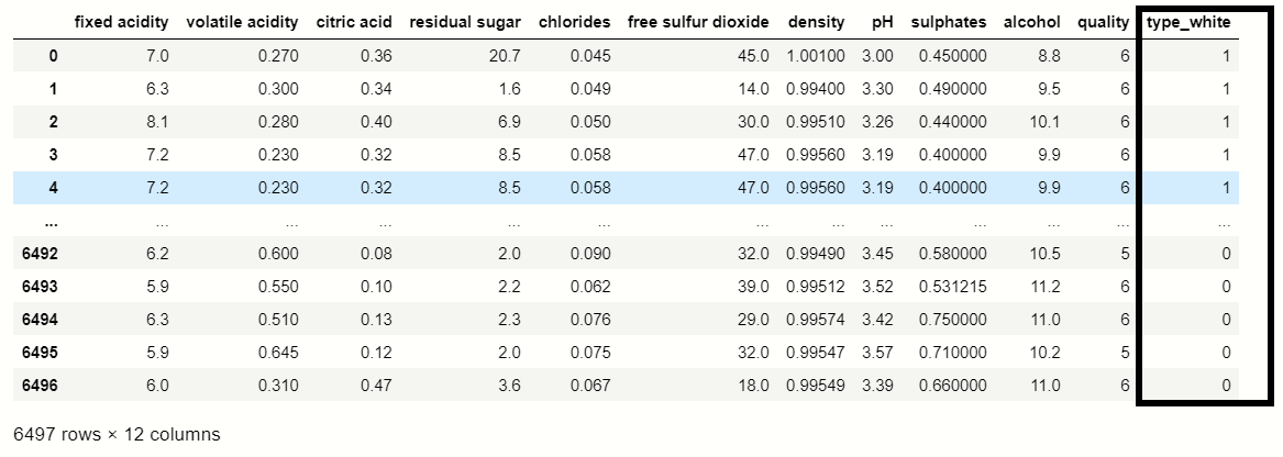
For the next step, we have to check what technical information contained in the data,
output:-
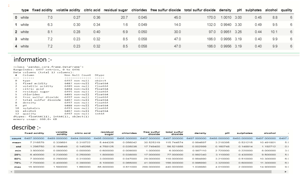
As we see in the above image, there is vital information on features and with this information, we will process our next work.
Visualization
We know that the “image speaks everything” here the visualization came into the work, we use visualization for explaining the data. In other words, we can say that it is a graphic representation of data that is used to find useful information.
df.hist(bins=25,figsize=(10,10))
# display histogram
plt.show()
output:-
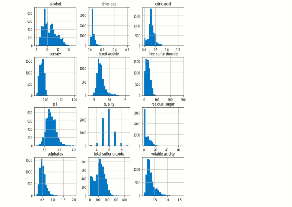
The above image reveals that how that data is easily distributed on features.
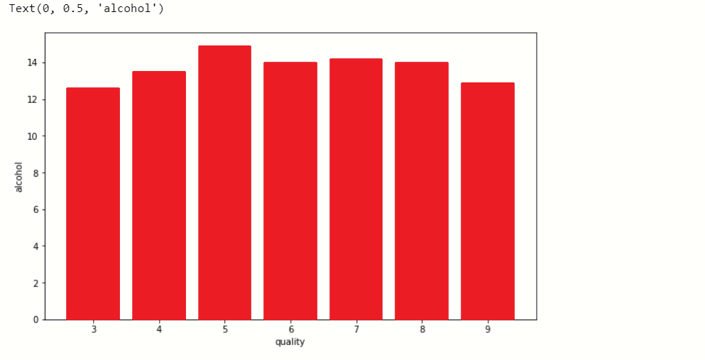
Now, we plot the bar graph in which we check what value of alcohol can able to make changes in quality.
plt.figure(figsize=[10,6])
# plot bar graph
plt.bar(df['quality'],df['alcohol'],color='red')
# label x-axis
plt.xlabel('quality')
#label y-axis
plt.ylabel('alcohol')
output:-
When we performing any machine learning operations then we have to study the data features deep, there are many ways by which we can differentiate each of the features easily. Now, we will perform a correlation on the data to see how many features are there they correlated to each other.
Correlation:-
For checking correlation we use a statistical method that finds the bonding and relationship between two features.
# ploting heatmap
plt.figure(figsize=[19,10],facecolor='blue')
sb.heatmap(df.corr(),annot=True)
output:-
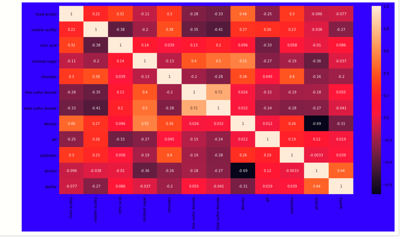
Now, we have to find those features that are fully correlated to each other by this we reduce the number of features from the data.
If you think that why we have to discard those correlated, because relationship among them is equal they equally impact on model accuracy so, we delete one of them.
for a in range(len(df.corr().columns)):
    for b in range(a):
        if abs(df.corr().iloc[a,b]) >0.7:
            name = df.corr().columns[a]
            print(name)
Here we write a python program with that we find those features whose correlation number is high, as you see in the program we set the correlation number greater than 0.7 it means if any feature has a correlation value above 0.7 then it was considered as a fully correlated feature, at last, we find the feature total sulfur dioxide which satisfy the condition.
So, we drop that feature
new_df=df.drop('total sulfur dioxide',axis=1)
Handle null values
In the dataset, there is so much notice data present, which will affect the accuracy of our ML model. In machine learning, there are many ways to handle null or missing values. Now, we will use them to handle our unorganized data.
new_df.isnull().sum()
We see that there are not many null values are present in our data so we simply fill them with the help of the fillna() function.
new_df.update(new_df.fillna(new_df.mean()))
with this, we handle only numerical variables value because, we fill mean() and mean value is not for categorical variables, so for categorical variables:-
# catogerical vars
next_df = pd.get_dummies(new_df,drop_first=True)
# display new dataframe
next_df
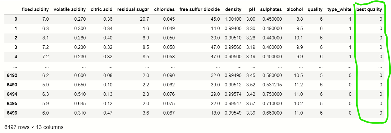
You were able to see that the get_dummies() function which is used for handling categorical columns, in this dataset ‘Type’ feature contains two types Red and White, where Red consider as 0 and white considers as 1.
df_dummies[''best quality''] = [ 1 if x>=7 else 0 for x in df.quality]
print(df_dummies)
Splitting dataset
Now we perform a split operation on our dataset:
from sklearn.model_selection import train_test_split
x_train,x_test,y_train,y_test = train_test_split(x,y,test_size=0.2,random_state=40)
Normalization
We do normalization on numerical data because our data is unbalanced it means the difference between the variable values is high so we convert them into 1 and 0.
#importing module
from sklearn.preprocessing import MinMaxScaler
# creating normalization object
norm = MinMaxScaler()
# fit data
norm_fit = norm.fit(x_train)
new_xtrain = norm_fit.transform(x_train)
new_xtest = norm_fit.transform(x_test)
# display values
print(new_xtrain)
Applying Model
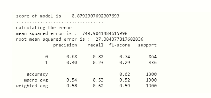
This is the last step where we apply any suitable model which will give more accuracy, here we will use RandomForestClassifier because it was the only ML model that gives the 88% accuracy which was considered as the best accuracy.
RandomForestClassifier:-
# importing modules
from sklearn.ensemble import RandomForestClassifier
from sklearn.metrics import classification_report
#creating RandomForestClassifier constructor
rnd = RandomForestClassifier()
# fit data
fit_rnd = rnd.fit(new_xtrain,y_train)
# predicting score
rnd_score = rnd.score(new_xtest,y_test)
print('score of model is : ',rnd_score)
# display error rate
print('calculating the error')
# calculating mean squared error
rnd_MSE = mean_squared_error(y_test,y_predict)
# calculating root mean squared error
rnd_RMSE = np.sqrt(MSE)
# display MSE
print('mean squared error is : ',rnd_MSE)
# display RMSE
print('root mean squared error is : ',rnd_RMSE)
print(classification_report(x_predict,y_test))
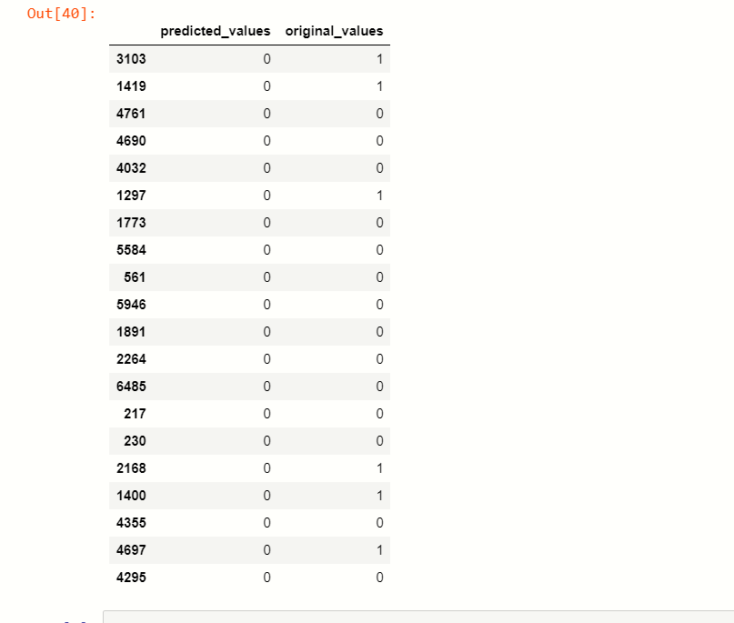
Now, we are at the end of our article, we can differentiate the predicted values and actual value.
x_predict = list(rnd.predict(x_test))
predicted_df = {'predicted_values': x_predict, 'original_values': y_test}
#creating new dataframe
pd.DataFrame(predicted_df).head(20)
Saving Model
At last, we save our machine learning model:
import pickle
file = 'wine_quality'
#save file
save = pickle.dump(rnd,open(file,'wb'))
So, at this step, our machine learning prediction is over.
End Notes
This is one of the interesting articles that I have written because it was on today’s current top technology machine learning, but I was used basic language to explain this article so, you can’t get difficulty on understanding.
If you have any question regarding this article then your will feel free to ask in the comment section below.
Thank you.
The media shown in this article are not owned by Analytics Vidhya and is used at the Author’s discretion.


Thank you for this well detailed explanation of using machine learning model to predict quality wines.... Please I'll like to know how you use the heat map to determine the correlation between the features... I don't understand the heat map Thanks
Hello Sir, thanks for the code and the explaination , but when i try to run this code in my Jupyter notebook it shows me an error "NameError Traceback (most recent call last) in 1 from sklearn.model_selection import train_test_split ----> 2 x_train,x_test,y_train,y_test = train_test_split(x,y,test_size=0.2,random_state=40) 3 df=x 4 #from sklearn.model_selection import train_test_split 5 #x_train,x_test,y_train,y_test = train_test_split(x,y,test_size=0.2,random_state=40) NameError: name 'x' is not defined" Can you please help me regarding my doubt . Thanks
Hello Sir , what are the social relevance of the project wine quality prediction. please reply..