Automated Machine Learning for Supervised Learning
This article aims to illustrate the concept of automated Machine Learning, commonly known as AutoML. Specifically, we will apply AutoML to a supervised learning problem involving tabular data, which includes regression and classification tasks. Please note that this article focuses exclusively on these types of problems and does not delve into other Machine Learning domains like clustering, dimensionality reduction, time series forecasting, Natural Language Processing, recommendation systems, or image analysis.
This article was published as a part of the Data Science Blogathon.
Table of contents
- Understanding the Problem Statement and Dataset
- Handling Missing Data and Outliers
- Feature Scaling for Improved Model Performance
- Enhancing Model Accuracy Through Feature Engineering
- Creating a Machine Learning Model
- Hyperparameter Tuning and Algorithm Exploration
- Ensemble Methods and Model Selection
- Saving and Reusing Models
- What is Automated Machine Learning or AutoML?
- Conclusion
- Frequently Asked Question
Understanding the Problem Statement and Dataset
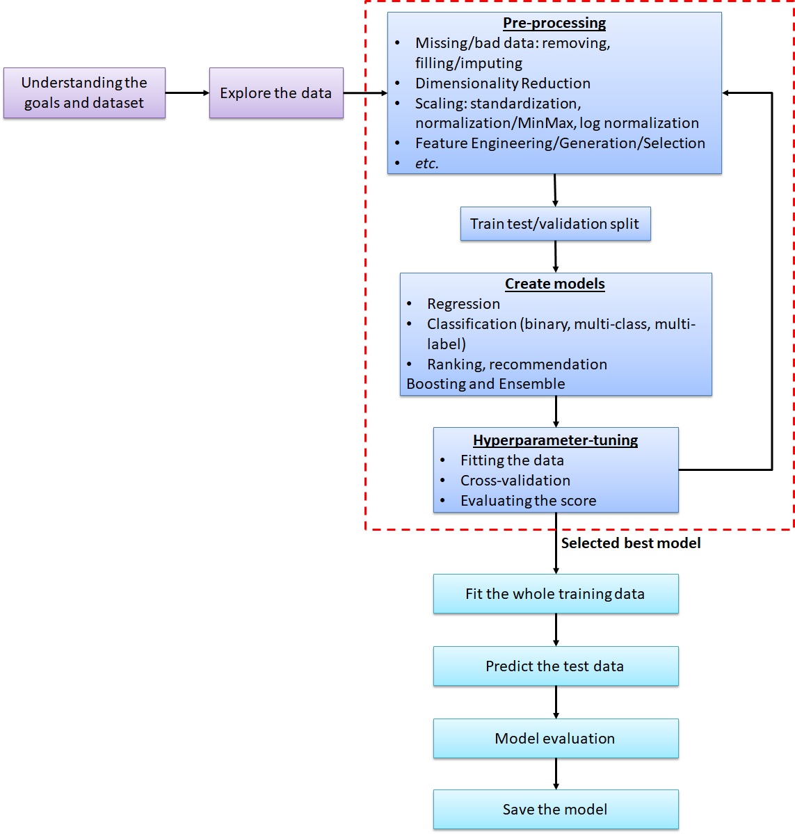
To prepare for AutoML, it’s crucial to begin with a solid understanding of the problem statement and the dataset. First, let’s establish a foundation by exploring conventional Machine Learning workflow. Once you have acquired the dataset and comprehended the problem statement, the next step is to define the task’s objective. In this article, our focus is primarily on regression and classification tasks, so ensure that the dataset is tabular in nature. Data formats such as time series, spatial, image, or text are not the primary areas of interest here.
Moving forward, delve into the dataset to gather essential insights, including:
- Descriptive statistics (count, mean, standard deviation, minimum, maximum, and quartiles), which can be obtained using .describe().
- Determine the data type of each feature using .info() or .dtypes.
- Explore the count of values within each feature through .value_counts().
- Identify the presence of null values using .isnull().sum().
- Assess feature correlations through correlation tests using .corr().
Handling Missing Data and Outliers
Users must decide between removing observations with missing data or applying data imputation techniques. Data imputation involves filling missing values with measures such as the average, median, a constant, or the most frequently occurring value. Additionally, users should pay close attention to identifying and handling outliers or erroneous data points, as they can introduce noise into the analysis.
Feature Scaling for Improved Model Performance
Feature scaling plays a pivotal role in data preprocessing, particularly for gradient descent- and distance-based Machine Learning algorithms. Its primary goal is to standardize the value range within each feature. This ensures that features with large values and low variance do not overshadow features with smaller values and higher variance. Various scaling methods, including standardization, normalization, and log normalization, can be employed to achieve this.
| Machine Learning Type | Algorithms |
| Gradient descent-based | Linear Regression, Ridge Regression, Lasso Regression, Elasticnet Regression, Neural Network (Deep Learning) |
| Distance-based | K Nearest Neighbors, Support Vector Machine, K-means, Hierarchical clustering |
| Tree-based | Decision Tree, Random Forest, Gradient Boosting Machine, Light GBM, Extreme Gradient Boosting, |
Enhancing Model Accuracy Through Feature Engineering
Feature engineering encompasses three key activities: generation, selection, and extraction. It involves creating new features that are expected to enhance predictive capabilities, removing low-importance features or noise, and generating new features by extracting partial information from existing ones. This step significantly influences model accuracy, as adding or removing features can lead to performance improvements and reduced computational overhead.
Creating a Machine Learning Model
In the journey of Machine Learning, selecting the right algorithm and building the model is a pivotal step. The algorithm requires training dataset features, a target or label feature, and certain hyperparameters as input arguments. Once the model is constructed, it is utilized to predict outcomes on validation or test datasets to assess its performance. To enhance the model’s performance, hyperparameter tuning is carried out. This process involves iteratively adjusting the hyperparameters of each Machine Learning algorithm until an optimal model is achieved. Model evaluation is based on scoring metrics, such as Root Mean Squared Error, Mean Squared Error, R2 for regression, and accuracy, Area Under the ROC Curve, or F1-score for classification problems. The model’s performance is assessed using cross-validation techniques.
Hyperparameter Tuning and Algorithm Exploration
After getting the optimum model with a set of hyperparameters, we may want to try other Machine Learning algorithms, along with the hyperparameter-tuning. There are many algorithms for regression and classification problems with their pros and cons. Different datasets have different Machine Learning algorithms to build the best prediction models. I have made notebooks containing a number of commonly used Machine Learning algorithms using the steps mentioned above. Please check it here:
| Tasks | Scorer | Notebook |
| Regression | RMSE, MAE, R2 | |
| Binary or Multiclass classification | Accuracy, F1-score |
Binary or Multi-class Classification-Accuracy-Titanic Survival |
| Binary classification (with probability) | AUC, accuracy, F1-score |
The datasets are provided by Kaggle. The regression task is to predict house prices using the parameters of the houses. The notebook contains the algorithms: Linear Regression, Ridge Regression, Lasso Regression, Elastic-net Regression, K Nearest Neighbors, Support Vector Machine, Decision Tree, Random Forest, Gradient Boosting Machine (GBM), Light GBM, Extreme Gradient Boosting (XGBoost), and Neural Network (Deep Learning).
Ensemble Methods and Model Selection
In scenarios where multiple models predict different outputs, the selection of the most appropriate model becomes crucial. One straightforward approach is to choose the model with the best score, whether it’s the lowest RMSE for regression or the highest accuracy for classification. Alternatively, ensemble methods can be employed, which involve using multiple diverse machine learning algorithms to predict the same dataset. The final prediction is typically determined through averaging predicted outputs in regression tasks or majority voting in classification tasks. Notably, Random Forest, Gradient Boosting Machine (GBM), and Extreme Gradient Boosting (XGBoost) are themselves ensemble methods, as they create decision trees from distinct subsets of training data.
Saving and Reusing Models
Once a satisfactory model is achieved, it can be saved for future use. The saved model can then be loaded into other notebooks to make consistent predictions or further analysis.
What is Automated Machine Learning or AutoML?
AutoML simplifies the laborious process of building Machine Learning models. While it doesn’t replace the need for understanding project goals, dataset exploration, and data preparation, it significantly streamlines tasks like data pre-processing, model selection, and hyperparameter tuning. Numerous AutoML packages exist, including Auto-Sklearn, which expedites these steps with minimal code, making Machine Learning more accessible.
# Install and import packages
!apt install -y build-essential swig curl
!curl https://raw.githubusercontent.com/automl/auto-sklearn/master/requirements.txt | xargs -n 1 -L 1 pip install
!pip install auto-sklearn
from autosklearn.classification import AutoSklearnClassifier
# Create the AutoSklearnClassifier
sklearn = AutoSklearnClassifier(time_left_for_this_task=3*60, per_run_time_limit=15, n_jobs=-1)
# Fit the training data
sklearn.fit(X_train, y_train)
# Sprint Statistics
print(sklearn.sprint_statistics())
# Predict the validation data
pred_sklearn = sklearn.predict(X_val)
# Compute the accuracy
print('Accuracy: ' + str(accuracy_score(y_val, pred_sklearn)))
Output
  Dataset name: da588f6e-c217-11eb-802c-0242ac130202
  Metric: accuracy
  Best validation score: 0.769936
  Number of target algorithm runs: 26
  Number of successful target algorithm runs: 7
  Number of crashed target algorithm runs: 0
  Number of target algorithms that exceeded the time limit: 19
  Number of target algorithms that exceeded the memory limit: 0
Accuracy: 0.7710593242331447

# Prediction results
print('Confusion Matrix')
print(pd.DataFrame(confusion_matrix(y_val, pred_sklearn)))
print(classification_report(y_val, pred_sklearn))
Output
Confusion Matrix
      0     1
0  8804  2215
1  2196  6052
              precision    recall  f1-score   support
           0       0.80      0.80      0.80     11019
           1       0.73      0.73      0.73      8248
    accuracy                           0.77     19267
   macro avg       0.77      0.77      0.77     19267
weighted avg       0.77      0.77      0.77     19267
The code is set to run for 3 minutes with no single algorithm running for more than 30 seconds. See, with only a few lines, we can create a classification algorithm automatically. We do not even need to think about which algorithm to use or which hyperparameters to set. Even a beginner in Machine Learning can do it right away. We can just get the final result. The code above has run 26 algorithms, but only 7 of them are completed. The other 19 algorithms exceeded the set time limit. It can achieve an accuracy of 0.771. To find the process of finding the selected model, run this line:
print(sklearn.show_models()).The following code is also Auto-Sklearn, but for regression work. It develops an autoML model to predict the House Prices dataset. It can find a model with RMSE of 28,130 from successful 16 algorithms out of the total 36 algorithms.
# Install and import packages
!apt install -y build-essential swig curl
!curl https://raw.githubusercontent.com/automl/auto-sklearn/master/requirements.txt | xargs -n 1 -L 1 pip install
!pip install auto-sklearn
from autosklearn.regression import AutoSklearnRegressor
# Create the AutoSklearnRegessor
sklearn = AutoSklearnRegressor(time_left_for_this_task=3*60, per_run_time_limit=30, n_jobs=-1)
# Fit the training data
sklearn.fit(X_train, y_train)
# Sprint Statistics
print(sklearn.sprint_statistics())
# Predict the validation data
pred_sklearn = sklearn.predict(X_val)
# Compute the RMSE
rmse_sklearn=MSE(y_val, pred_sklearn)**0.5
print('RMSE: ' + str(rmse_sklearn))
Output
Dataset name: 71040d02-c21a-11eb-803f-0242ac130202
  Metric: r2
  Best validation score: 0.888788
  Number of target algorithm runs: 36
  Number of successful target algorithm runs: 16
  Number of crashed target algorithm runs: 1
  Number of target algorithms that exceeded the time limit: 15
  Number of target algorithms that exceeded the memory limit: 4
RMSE: 28130.17557050461

# Scatter plot true and predicted values
plt.scatter(pred_sklearn, y_val, alpha=0.2)
plt.xlabel('predicted')
plt.ylabel('true value')
plt.text(100000, 400000, 'RMSE: ' + str(round(rmse_sklearn)))
plt.text(100000, 350000, 'MAE: ' + str(round(mean_absolute_error(y_val, pred_sklearn))))
plt.text(100000, 300000, 'R: ' + str(round(np.corrcoef(pred_sklearn, y_val)[0,1],2)))
plt.show()
Output
# Scatter plot true and predicted values
plt.scatter(pred_sklearn, y_val, alpha=0.2)
plt.xlabel('predicted')
plt.ylabel('true value')
plt.text(100000, 400000, 'RMSE: ' + str(round(rmse_sklearn)))
plt.text(100000, 350000, 'MAE: ' + str(round(mean_absolute_error(y_val, pred_sklearn))))
plt.text(100000, 300000, 'R: ' + str(round(np.corrcoef(pred_sklearn, y_val)[0,1],2)))
plt.show()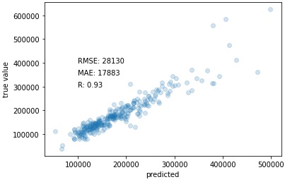
Conclusion
In conclusion, Automated Machine Learning (AutoML) revolutionizes the landscape of supervised learning. It simplifies and accelerates the process, allowing data scientists to focus on problem-solving rather than coding intricacies. AutoML packages like Auto-Sklearn make advanced Machine Learning accessible with minimal effort, opening up new possibilities for efficient model development and deployment. Embracing AutoML empowers practitioners to harness the full potential of Machine Learning for various applications.
Frequently Asked Question
A. AutoML automates Machine Learning tasks, including data preprocessing, model selection, and hyperparameter tuning, streamlining the model development process.
A. AutoML solutions vary, with options ranging from free, open-source tools to paid services, offering flexibility based on users’ needs and budgets.
A. One disadvantage is its potential lack of customization compared to manual model development, which may limit fine-tuning for specific requirements.
A. Yes, data scientists frequently use AutoML tools to save time, explore diverse algorithms, and efficiently develop models.
The media shown in this article are not owned by Analytics Vidhya and are used at the Author’s discretion.


