Outliers Detection Using IQR, Z-score, LOF and DBSCAN

This article was published as a part of the Data Science Blogathon.

Introduction

Are you dealing with outliers? Thinking about which method is better for detecting outliers for skewed or normally distributed data? Which methods will work well if data density is not the same through the dispersion? Identification of outliers? Etc. 

Guys, this article will help you to get many such questions answered along with practical applications, no matter if you are doing a data cleaning process before conducting EDA,/ passing data to a Machine learning model, or performing any statistical test.

What are Inliers and Outliers?

Outliers are values that seem excessively different from most of the rest of the values in the given dataset. Outliers could normally exist due to new inventions (true outliers), development of new patterns/phenomena, experimental errors, rarely occurring incidents, anomalies, incorrectly fed data due to typographical mistakes, failure of data recording systems/components, etc. However, all outliers are not bad; some reveal new information. Inliers are all the data points that are part of the distribution except outliers. 

Outlier’s Identification

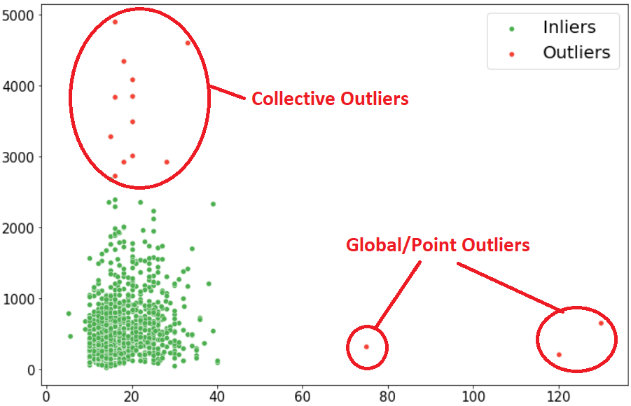
Global or Point Outliers:  This is a single value/data point that deviates from the distribution, and most outlier detection methods are usually intended to detect point / global outliers. Ref. Fig-1.
Collective Outliers: When a Group of datapoint deviates from the distribution, it is called a collective outlier. It is completely subjective to interpret their relevance according to the specific domain. Also, collective outliers show the formation of new phenomena or development. Ref. 

Contextual Outliers: These are specific conditions based on where the interpretation of its relevance becomes (i.e., the usual temperature in Leh during winter goes near 9°C which is the rarest phenomenon in Ahmedabad, Gujarat), Punctuation symbols while attempting text analysis,  background noise single while doing speech recognition, etc.)

For ease of understanding, I have considered a real case study on steel scrap sales over three years.

Real Case Example of Outliers

Considering a real-case scenario of Steel Sheet Scrap Rate (Rs/Kg) sold across India from 2018 to 2022 has been captured to understand the statistics and predict the price in the future. Still, before doing that, as part of the data-cleaning process, we want to understand the presence of an outlier and its weightage accordingly. 

Importing important libraries to load the dataset and conduct further analysis:

import pandas as pd
import numpy as np
import matplotlib.pyplot as plt
import seaborn as sns
import scipy.stats as st
%matplotlib inline
import warnings
warnings.filterwarnings('ignore')

df=pdf.read_excel("scrap_data.xlsx", skiprows=2)
df.head(), print('shape of data:',df.shape)

To understand the trend, I have tried to plot line plot on two main independent

variables (‘Scrap Rate’ and ‘Scrap Weight’)  with ref. to their date of sale. 

plt.figure(figsize =(15,5))
plt.subplot(1,2,1)
sns.lineplot(x=df['Job Start Date'], y=df['Rate in Rs./Kg.'], color='r')
plt.title("Steel Scrap Rate (Rs/Kg)", fontsize=20)
plt.xlabel('Date')
plt.subplot(1,2,2)
sns.lineplot(x=df['Job Start Date'], y=df['Scrape Sale Qty.'], color='b')
plt.title("Steel Scrap Weight (Rs/Kg)", fontsize=20)
plt.xlabel('Date')

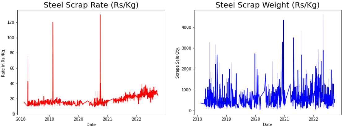
Looking at the trend in the Scrap Rate feature, we understand that there were sudden spikes in rates crossing 120 Rs/kg, indicating anomalies as the scrap rate must be the same and increase or decrease gradually. However, in the case of Scrap weight, depending on the size of a construction project, scrap generated at the end of closing the project may be high or low in volume anytime.

Let’s try applying the different methods of detecting and treating outliers:

Inter Quartile Range (IQR)

IQR measures variability by dividing the dataset into four equal quartiles. First, the entire data is to be sorted in ascending order, and then splitting it into four equal quartiles called Q1, Q2, Q3, and Q4, which can be calculated using the following equation. IQR Method is best suited when the data forms a skewed distribution.

The first Quartile (Q1) divides the smallest 25% of the values from the other 75% that are larger.

Q1 = (n+1)/4 Ranked Value (25th Percentile)

The Third quantile (Q3) divides the smallest 75%  of the values from the largest 25%.

Q3 = 3(n+1)/4 Ranked Value (75th Percentile)

IQR (Inter Quantile Range) = Q3– Q1

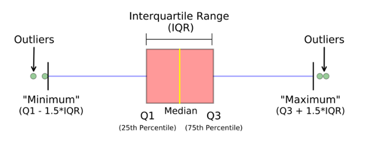
So outliers can be considered any values which are greater than Upper Bound Limit (Q3+1.5*IQR) and less than Lower Bound Limit (Q1-1.5*IQR) in the given dataset.

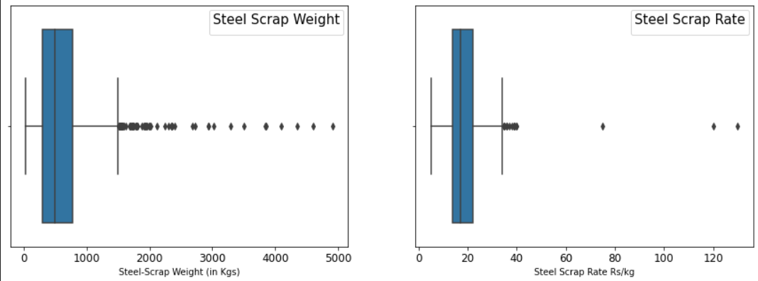
Let’s plot Boxplot to know the presence of outliers;

plt.figure(figsize=(15,5))
plt.subplot(1,2,1)

sns.boxplot(df['Scrape Sale Qty.'])
plt.xticks(fontsize = (12))
plt.xlabel('Steel-Scrap Weight (in Kgs)')
plt.legend (title="Steel Scrap Weight", fontsize=10, title_fontsize=15)

plt.subplot(1,2,2)
sns.boxplot(df['Rate in Rs./Kg.'])
plt.xlabel('Steel Scrap Rate Rs/kg')
plt.xticks(fontsize =(12));
plt.legend (title="Steel Scrap Rate", fontsize=10, title_fontsize=15);

To make the calculation faster, I have created a function to derive Inter-Quartile-Range (IQR), Lower Fence, and Upper Fence and added conditions either to drop them or fill them with upper or lower values, respectively. 

def identifying_treating_outliers(df,col,remove_or_fill_with_quartile):

  q1=df[col].quantile(0.25)

  q3=df[col].quantile(0.75)

  iqr=q3-q1

  lower_fence=q1-1.5*(iqr)

  upper_fence=q3+1.5*(iqr)

  print('Lower Fence;', lower_fence)

  print('Upper Fence:', upper_fence)

  print('Total number of outliers are left:', df[df[col]  upper_fence].shape[0])

  if remove_or_fill_with_quartile=="drop":

    df.drop(df.loc[df[col]<lower_fence].index,inplace=True)

    df.drop(df.loc[df[col]>upper_fence].index,inplace=True)

  elif remove_or_fill_with_quartile=="fill":

    df[col] = np.where(df[col] < lower_fence, lower_fence, df[col])

    df[col] = np.where(df[col] > upper_fence, upper_fence, df[col])

Applying the Function to the Scrap Rate and Scrap Weight column:

identifying_treating_outliers(df,'Scrape Sale Qty.','drop')
identifying_treating_outliers(df,'Rate in Rs./Kg.','drop')

DF shape before Application of Function : (1001, 5)

DF Shape after Application of Function : (925, 5)

Plotting Boxplot to check the status of outliers after applying the ‘indentifying_treating_outliers’ function: 

plt.figure(figsize=(15,5))

plt.subplot(1,2,1)
sns.boxplot(df['Scrape Sale Qty.'])
plt.xticks(fontsize = (12))
plt.xlabel('Steel-Scrap Weight (in Kgs)')
plt.legend (title="Steel Scrap Weight", fontsize=10, title_fontsize=15)

plt.subplot(1,2,2)
sns.boxplot(df['Rate in Rs./Kg.'])
plt.xlabel('Steel Scrap Rate Rs/kg')
plt.xticks(fontsize =(12));
plt.legend (title="Steel Scrap Rate", fontsize=10, title_fontsize=15);

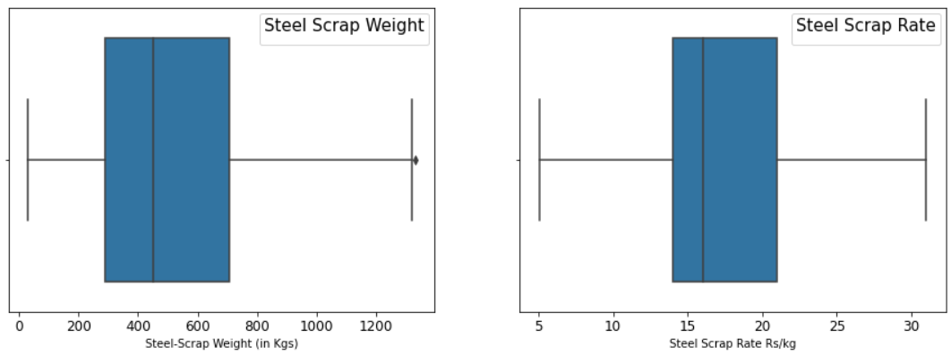
Using IQR Method, we have dropped 15 data points from Scrap Rate (Rate > 34 Rs/kg) and 65 data points from Scrap Weight (>1503 kg), respectively. The total number of observations dropped is 76.

Z-score Method

TheZ-score of the values is the difference between that value and the mean, divided by the standard deviation. Z-Scores help identify outliers by values if a particular data point has a Z-score value either less than -3 or greater than +3.Z score can be mathematically expressed as;

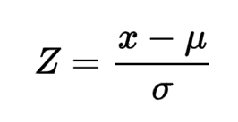
= particular value, =mean, =standard deviation

Below pic expresses the transformation of data from normal distribution to a standard normal distribution using a Z-score is given here for ref.

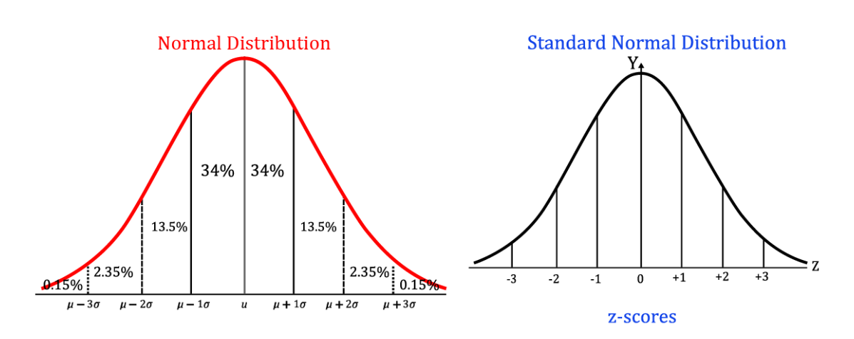
In our dataset, we will apply the Zscore for outliers with a Zscore of more than +3 and less than -3. Just a few lines of code will help us get Zscore, and we can see the differences using the distribution plot (before and after).

# Applying Zscore in Scrap Rate column defining dataframe by dfn

zr = st.zscore(df['Rate in Rs./Kg.'])

dfn = df[(zr-3)]

# Applying Zscore in Steel Weight Column defining dataframe by dfnf

zw= st.zscore(dfn['Scrape Sale Qty.'])

dfnf = dfn[(zw-3)]

plt.figure(figsize=(12,5))

plt.subplot(1,2,1)
sns.distplot(df['Rate in Rs./Kg.'])
plt.title('Z Score Plot Before Removing Outlier',fontsize=15)

plt.subplot(1,2,2)
sns.distplot(st.zscore(dfn['Rate in Rs./Kg.']))
plt.title('Z Score Plot After Removing Outlier',fontsize=15)

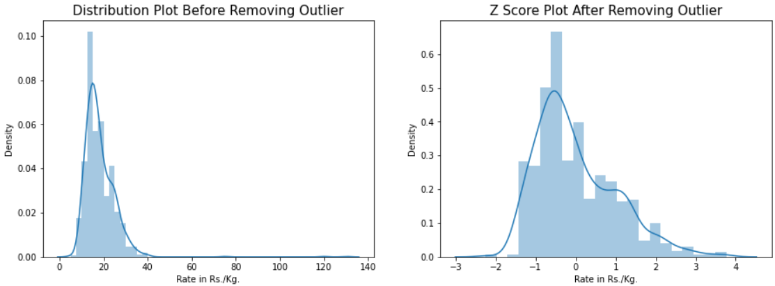
Our data forms a Positive Skewed distribution (skewness value- 0.874) which cannot be considered approximately normally distributed through the above plot. Significant improvement can be seen comparing the plot shown before and after applying Zscore.

print('before df shape', df.shape)

print('After df shape for Observation dropped in Scrap Rate', dfn.shape)

print('After df shape for observation dropped in weight', dfnf.shape)

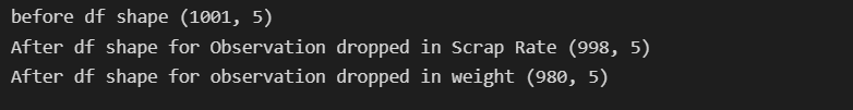
Using the Z Score method, in Scrap Rate and Scrap Weight columns, we have dropped 21 data points (3 from Scrap Rate and 18 from Scrap Weight) with Zscore -3.

Local Outliers Finder (LOF)

Local Outlier Finder is an unsupervised machine learning technique to detect outliers based on the closest neighborhood density of data points and works well when the spread of the dataset (density) is not the same. LOF basically considers  K-distance (distance between the points) and K-neighbors (set of points lies in the circle of K-distance (radius)). Ref. detailed documentation: SK-Learn  Library.

Lof takes two major parameters into consideration (1) n_neighbors: The number of neighbors which has a default value of 20 (2) Contamination: the proportion of outliers in the given dataset which can be set ‘auto’ or float values (0, 0.02, 0.005).

Importing important libraries and defining model

from sklearn.neighbors import LocalOutlierFactor

d2 = df.values #converting the df into numpy array

lof = LocalOutlierFactor(n_neighbors=20, contamination='auto')
good = lof.fit_predict(d2) == 1
plt.figure(figsize=(10,5))
plt.scatter(d2[good, 1], d2[good, 0], s=2, label="Inliers", color="#4CAF50")
plt.scatter(d2[~good, 1], d2[~good, 0], s=8, label="Outliers", color="#F44336")
plt.title('Outlier Detection using Local Outlier Factor', fontsize=20)
plt.legend (fontsize=15, title_fontsize=15)

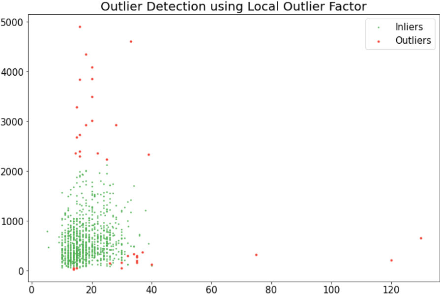
In our case, I have set contamination as ‘auto’ (see the above plot) to see the result and found LOF is not performing that well as my data spread (density) is not deviating much. Also, I tried different Contamination values of 0.005, 0.01, 0.02, 0.05, and 0.09 but the performance was not that well.

Density-Based Spatial Clustering for Application with Noise (DBSCAN)

When our dataset is large enough that have multiple numeric features (multivariate) then it becomes difficult to handle outliers using IQR, Zscore, or LOF. Here SK-Learn library DBSCAN comes to the rescue to allow us to handle outliers for the Multi-variate datasets.

DBSCAN considers two main parameters (as mentioned below) to form a cluster with the nearest data point and based on the high or low-density region, it detects Inliers or outliers.

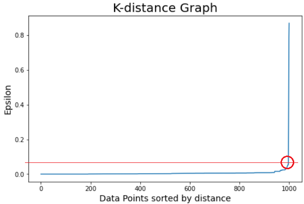
(1) Epsilon (Radius of datapoint that we can calculate based on k-distance graph)

(2) Min_samples (number of data points to be considered in the Epsilon (radius) which depends on domain knowledge or expert advice)

However, in our case, we don’t have more than 5 features and we have just selected two important numeric features out of them to apply our learnings and visualize the same. Due to the technology & human brain’s limitation in visualizing the Multi-dimensional data altogether at the moment, we are applying DBSCAN to our dataset.

Importing the libraries and fitting the model. To nullify the noise in the data set, we have u normalized the data using Min-Max Scaler.

from sklearn.cluster import DBSCAN
from sklearn.preprocessing import MinMaxScaler
mms = MinMaxScaler()
df[['Scrape Sale Qty.','Rate in Rs./Kg.']] = mms.fit_transform(df[['Scrape Sale Qty.','Rate in Rs./Kg.']])
df.head()
from sklearn.neighbors import NearestNeighbors
neigh = NearestNeighbors(n_neighbors=2)
nbrs = neigh.fit(df[['Scrape Sale Qty.', 'Rate in Rs./Kg.']])
distances, indices = nbrs.kneighbors(df[['Rate in Rs./Kg.', 'Rate in Rs./Kg.']])
# Plotting K-distance Graph
distances = np.sort(distances, axis=0)
distances = distances[:,1]

plt.figure(figsize=(8,5))
plt.plot(distances)
plt.title('K-distance Graph',fontsize=20)
plt.xlabel('Data Points sorted by distance',fontsize=14)
plt.ylabel('Epsilon',fontsize=14)
plt.show()

model = DBSCAN(eps = 0.08, min_samples = 10).fit(data)
colors = model.labels_
plt.figure(figsize=(10,7))
plt.scatter(df['Rate in Rs./Kg.'], df['Scrape Sale Qty.'], c = colors)
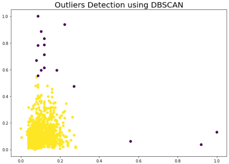
plt.title('Outliers Detection using DBSCAN',fontsize=20)

DBSCAN technique has efficiently detected the significant outliers using Density-Based Spatial Clustering and can be seen in the below plots.

 

Conclusion

Here we have gone through Four Methods of Detecting the outliers from our dataset, found their implementation on Real-worlds Dataset, and observed different outcomes. However, applications of these methods also depend on the size, spread, distribution, and context of the dataset (univariate, bivariate, or multivariate). All these techniques have certain advantages and disadvantages.

Finally, outliers treatment is to be done judiciously, especially as per the advice of subject matter experts and in the context of business scenarios, especially when dealing with a limited/small-size dataset. In most cases dropping these outliers is one of the options but based on the context of business, it needs to be replaced or dropped with domain knowledge.

The media shown in this article is not owned by Analytics Vidhya and is used at the Author’s discretion.

Shailesh Shukla 14 Nov 2022